ABAI Webinar

Modeling Individual and Group Outcomes:

A (very brief) Introduction to Mixed Effects Models

For Behavior Analysts, Behavioral Scientists, and Researchers

About Me

Background

PhD in Behavioral Psychology, University of Kansas (Derek Reed)
Graduate Research Assistant, Center for Research Methods and Data Analysis (Paul Johnson)
Postdoctoral Fellow, Virginia Tech (Mikhail Koffarnus and Warren Bickel)
Assistant Professor, University of Kentucky College of Medicine
Data Scientist, Advocates for Human Potential

Things I Do

Advocates for Human Potential

Create and implement data pipelines, generate data insights via modeling, full stack app development

codedbx

Serve as a research and statistical consultant, conduct analyses, and generate reports
Build open-source tools: R packages (beezdemand, beezdiscounting) and the R Shiny web app shinybeez
Built the 27-Item Monetary Choice Questionniare Automated Scorer
Authored 70+ peer-reviewed publications
More about me and my work at codedbx.com

Brent Kaplan headshot

Acknowledgements and Disclaimers

None of what I am talking about today reflects the views or opinions of Advocates for Human Potential
These are my own ideas and thoughts, heavily informed by my own experiences, things that I’ve read, and people that I’ve talked to
Have to acknowledge many of the people who have shaped my thinking and informed my approaches to data analysis
People including: Derek Reed, Paul Johnson, Mikhail Koffarnus, Warren Bickel, Chris Franck, Brady DeHart, Steve Hursh, and others
Also I’m not a statistician nor am I a practicing applied behavior analyst, so take everything I say with skepticism

What you will NOT learn

A full cookbook of model fitting in R (or other software)
Exhaustive diagnostic procedures and model selection strategies
How to interpret every model coefficient and how to use them to make predictions
Deep mathematical derivations

What I hope you will learn

Recognize when mixed-effects models are appropriate
Distinguish fixed vs. random effects (with intuition)
Identify data scenarios (e.g. repeated measures or hierarchical datasets) where mixed-effects models are an appropriate analytic approach
Explain how incorporating random effects in a model accounts for individual differences and addresses limitations of traditional analyses that rely on data aggregation
Learn how they apply to single-case designs and behavioral economic data
Gain basic intuition through visual examples
Leave with resources and confidence to explore further

Deep reflection

When confronted with some data, what do most behavior analysts or applied behavioral scientists reach for?

Visual inspection?
Descriptive statistics?

Maybe if you’re feeling brave, a statistical test?

T-test?
ANOVA?
Regression?

Deep reflection

Sometimes those tools are exactly right.

But sometimes they’re not sufficient in and of themselves.

And sometimes they’re not even the right tools at all.

A small simulated dataset

Imagine measuring some behavior over time for multiple subjects. Each subject is in a different condition and we want to model what affect the condition has on behavior across sessions.

If we are feeling brave…

We could fit a linear regression by condition, and then compare the slope and intercept between conditions
Typical linear regression: \(y = Intercept + Slope * x\)

m_lm <- lm(response ~ session + condition, data = dat)
dat$fitted_lm <- predict(m_lm)

p +
  geom_line(data = dat, aes(y = fitted_lm, color = condition))

Looks pretty good…

What does our output say?

summary(m_lm)


Call:
lm(formula = response ~ session + condition, data = dat)

Residuals:
    Min      1Q  Median      3Q     Max 
-4.4349 -1.5101 -0.1005  1.4455  4.6365 

Coefficients:
            Estimate Std. Error t value Pr(>|t|)    
(Intercept) 24.67256    0.47151  52.326  < 2e-16 ***
session     -0.48729    0.03254 -14.976  < 2e-16 ***
condition2   1.95819    0.45958   4.261 4.16e-05 ***
condition3   2.64218    0.45958   5.749 7.39e-08 ***
---
Signif. codes:  0 '***' 0.001 '**' 0.01 '*' 0.05 '.' 0.1 ' ' 1

Residual standard error: 2.055 on 116 degrees of freedom
Multiple R-squared:  0.6914,    Adjusted R-squared:  0.6834 
F-statistic: 86.64 on 3 and 116 DF,  p-value: < 2.2e-16

We know how the overall effect of condition affects behavior across session, but that’s all we really know. We don’t know about how each subject responds and their trajectory.

Ok, easy. Let’s just fit a line to each subject!

Both of these are considered fixed-effect only models because the parameters we estimate are fixed either across subjects or fixed within subjects.

Ok, easy. Let’s just fit a line to each subject!

Fixed effects definition

Fixed effects are assumed constant in the broader population from which the observed data are drawn. The sample data are used to produce estimates of these parameters, and the resulting estimates have with some degree of imprecision (i.e., standard error).

Another way to think about it is a “pooled” model (all the data points are pooled together; i.e., “fit to group”) vs. no pooling model (each subject has its own data points; i.e., “two-stage”). The latter considered “amnesic” models because they ignore information from other subjects (see McElreath, 2020).
Overfitting risk: no borrowing of strength → noisy subject-level slopes
Inflated uncertainty: two-stage standard errors often understate uncertainty for population questions

Enter Mixed Effects Modeling

Mixed-effects models definition

A mixed-effects model (also called a multilevel or hierarchical model) is a regression model that includes both fixed effects and random effects. In practical terms, it allows some parameters to vary by group or subject while estimating overall effects.

Why use them? They handle nested data or repeated measures by modeling variability at multiple levels (e.g., within-individual and between-individual). This means we can account for individual differences without losing them in the analysis.
Key idea: Unlike a simple one-size-fits-all approach, mixed models capture each subject’s story within the bigger story. Think of each participant as a short story within an anthology: the anthology tells a general narrative (fixed effects) while each story has its own nuances (random effects).

Let’s see them in action

One flavor that we can specify is what is called a random intercepts model (or a random effects model).

m_ri <- lmer(
  response ~ session + condition + (1 | subject),
  data = dat
)

Notice we use the lmer package here instead of the lm package. In this code, we are specifying our outcome as a function of session and condition (just like in the fixed-effects only model), but now we are specifying we want the intercept to be random (i.e., different for each subject).

Let’s see them in action

However, this model assumes that the slope is constant across subjects, so we may want to add a random slope term to the model.

Let’s see them in action

m_rirs <- lmer(
  response ~ session + condition + (session | subject),
  data = dat
)

In this code, we are specifying our outcome as a function of session and condition (just like in the fixed-effects only model and our random intercepts model), but now we are specifying we want the intercept and the slope (session) to be random (i.e., different for each subject).

Let’s see them in action

Fixed vs. Random Effects (Simply)

Fixed effect

An effect that is constant across individuals (e.g., a treatment effect assumed to be the same for everyone). It’s something we explicitly estimate for the population.

Random effect

An effect that varies across individuals or clusters. It’s not a single estimate but a distribution. For example, each subject can have their own intercept (starting level) or slope (trend), and these are assumed to be drawn from some population distribution. The larger the random effect, the model is capturing more variability between individuals/groups.

Fixed vs. Random Effects (Simply)

\(y_{ij} = \beta_0 + \beta_1 \, \text{time}_{ij} + u_{0j} + u_{1j}\,\text{time}_{ij} + \varepsilon_{ij}\)

(\(\beta\)): fixed effects (population)
(\(u\)): random effects (subject/cluster deviations)
(\(\varepsilon\)): residual/error

Metaphor

Fixed effects = the overall recipe

Random effects = each chef’s personal twist on that recipe.

We model the general effect and the individual deviations.

Ok, but why should I care?

What you mean to ask is when should I consider using a mixed effects model?

Take this scenario for example (from DeHart & Kaplan, 2019):

Or this scenario (from Krzywinski et al., 2014):

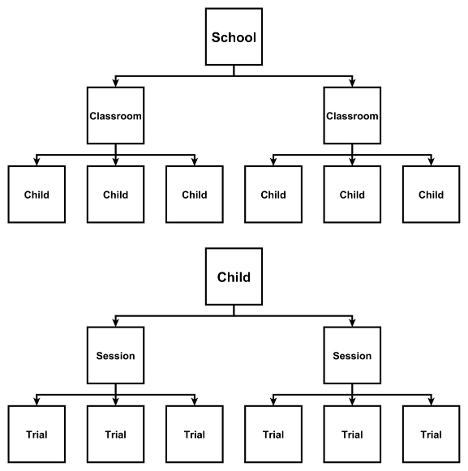
Hierarchical (nested) data structure: Illustration of three-level hierarchy (Level 3 = school/individual, Level 2 = classrooms/sessions, Level 1 = children/trials). In this illustration, each school (or individual) includes multiple classrooms (or sessions), and each classroom or session has multiple observations (children or trials). Such nesting means observations within a classroom are (probably) more alike than observations from different classrooms. Likewise, observations within a session are (probably) more alike than observations from different sessions.

However, not all data are purely nested. Sometimes, the same observation belongs to multiple grouping factors that are not contained within each other — for example, students nested within both classrooms and teachers, where teachers teach multiple classrooms, and classrooms have multiple teachers across time. This is known as a crossed-effects (or non-nested) design.

Mixed-effects models can handle these too — by estimating random effects for each grouping factor (e.g., classroom and teacher) simultaneously, recognizing that variability arises from both sources independently.

Modeling crossed factors example:

\(y_{it} \sim \beta_0 + \beta_1 \text{time}_{it} + (1|\text{student}_i) + (1|\text{teacher}_t)\)

(Students and teachers are crossed; each contributes its own random intercept.)

Some big picture benefits of mixed-effects models

As we just saw in our hierarchical diagram, many studies in behavioral science involve multiple participants with repeated observations (e.g., multiple baseline designs, ABAB reversal/withdrawal designs).
Traditional statistical tests may ignore or not account for the nonindependence of repeated observations within the study. Ignoring these characteristics can lead to biased inferences.
Mixed models can incorporate these types of correlations (implicitly or explicitly).

In behavioral science, simply averaging data (or using only traditional ANOVA/t-tests) can hide important patterns. Conventional stats often aggregate group and/or time variability into means, effectively washing out individual differences.
For example, you might conclude an intervention has a moderate effect by averaging, even if one subgroup improved greatly and another not at all.
Single-case designs often emphasize visual analysis for exactly this reason: averaging across participants can be misleading.
Mixed-effects models address this by incorporating random effects, which quantify each subject’s variability without eliminating it, so the model can predict both group-level and individual behavior.

In an earlier example, we treated condition as a fixed effect with three different levels. Each fixed effect level we estimate uses up one degree of freedom. When we have many fixed effects, we use up many degrees of freedom, which reduces our power to detect effects.
In a mixed-effects model, we have a single degree of freedom for each random effect, which allows us to detect effects with greater power.

Applications in Behavior Analysis: SCEDs

Single-Case Experimental Designs (SCEDs): These often involve a small number of subjects with many repeated observations. Traditional analyses might rely on visual inspection or simple statistics to summarize the data.
Mixed-effects models let us model data from multiple participants while accounting for individual differences. We get more statistical power than analyzing each case separately, but we still respect that each case may respond differently.

Example: Dehart & Kaplan (2019)

Fixed effects of condition (control, experimenter, child) and session (interaction between condition and session)
Random intercept for child, and random slope of condition and session to allow for individual variation in the rate of selections over sessions by condition
In that paper, we describe some additional things, mainly use of a zero-inflated negative binomial link function

Example: Dehart & Kaplan (2019)

glmm_model <- glmmTMB(
  frequency ~
    condition * I(log(session)) + (condition + I(log(session)) || child),
  data = Final,
  ziformula = ~ condition * I(log(session)),
  family = nbinom2(),
  REML = FALSE
)

 Family: nbinom2  ( log )
Formula:          frequency ~ condition * I(log(session)) + (condition + I(log(session)) |
    child)
Zero inflation:             ~condition * I(log(session))
Data: Final

      AIC       BIC    logLik -2*log(L)  df.resid
   1240.6    1327.6    -597.3    1194.6       302

Random effects:

Conditional model:
 Groups Name                  Variance Std.Dev.  Corr
 child  (Intercept)           1.936904 1.3917
        conditionExperimenter 2.220070 1.4900    -0.94
        conditionChild        2.428950 1.5585    -0.98  0.86
        I(log(session))       0.004748 0.0689     0.61 -0.31 -0.75
Number of obs: 325, groups:  child, 15

Dispersion parameter for nbinom2 family (): 7.14e+12

Conditional model:
                                      Estimate Std. Error z value Pr(>|z|)
(Intercept)                            -0.6837     0.5012  -1.364 0.172546
conditionExperimenter                   2.3890     0.5287   4.519 6.23e-06 ***
conditionChild                          2.6842     0.5377   4.992 5.98e-07 ***
I(log(session))                        -0.6644     0.1775  -3.743 0.000182 ***
conditionExperimenter:I(log(session))   0.3479     0.1917   1.815 0.069525 .
conditionChild:I(log(session))          0.8851     0.1822   4.857 1.19e-06 ***
---
Signif. codes:  0 ‘***’ 0.001 ‘**’ 0.01 ‘*’ 0.05 ‘.’ 0.1 ‘ ’ 1

Zero-inflation model:
                                        Estimate Std. Error z value Pr(>|z|)
(Intercept)                              -3.2020     3.8459  -0.833    0.405
conditionExperimenter                    -1.0667     4.2251  -0.252    0.801
conditionChild                          -14.6832  1972.5675  -0.007    0.994
I(log(session))                          -0.1825     2.6053  -0.070    0.944
conditionExperimenter:I(log(session))     1.0991     2.7331   0.402    0.688
conditionChild:I(log(session))           -4.5532 12007.7784   0.000    1.000

Example: Dehart & Kaplan (2019)

Takeaways:

Mixed models produced results consistent with the usual visual analysis, while providing a statistical framework that predicts individual behavior without requiring data aggregation
By including random effects for each subject, the model captured variability between children (each child had their own intercept reflecting baseline preference).
Mixed models as an additional tool to visual inspection.
Mixed models should correspond to visual inspection. When they don’t, this discrepancy should be investigated to determine if this is a shortcoming of the model or of visual inspection.
General guidance for minimum number of “clusters” (e.g., participants in a single subject design) - about 20 clusters with about 20 observations per cluster to minimize bias.

Example: Dehart & Kaplan (2019)

For more, see the full paper (also available at codedbx.com)

Applications in Behavioral Economic Demand and Discounting

Applications: Behavioral Economic Demand

Behavioral economic demand curves (e.g., how consumption of a reinforcer changes as price/cost increases) are often fit for each subject or at the group level. Mixed models bring a modern approach here.
Traditionally, demand data might be analyzed with either a “fit-to-group” method (fit one curve to aggregated data) or a “two-stage” method (fit each individual separately, then compare parameters). Both have drawbacks, which we have discussed. The first ignores individual differences, the second ignores shared patterns and can have less power.
In a paper I published (Kaplan et al. (2021)), I provided an introduction to mixed-effects modeling for demand data as an improvement over those methods.
Notable benefits include providing simultaneous population-level estimates (with better standard errors) and individual-level predictions, while handling things like non-systematic data points and covariates.
For instance, in a demand study, each subject’s demand curve (e.g., parameters like \(Q_0\) or \(\alpha\)) can be a random effect. The mixed model might find overall fixed effects for these parameters and how much individuals deviate (random effects). This means we can predict demand for any given individual while also being able to describe how the group responds as a whole.

Applications: Behavioral Economic Demand

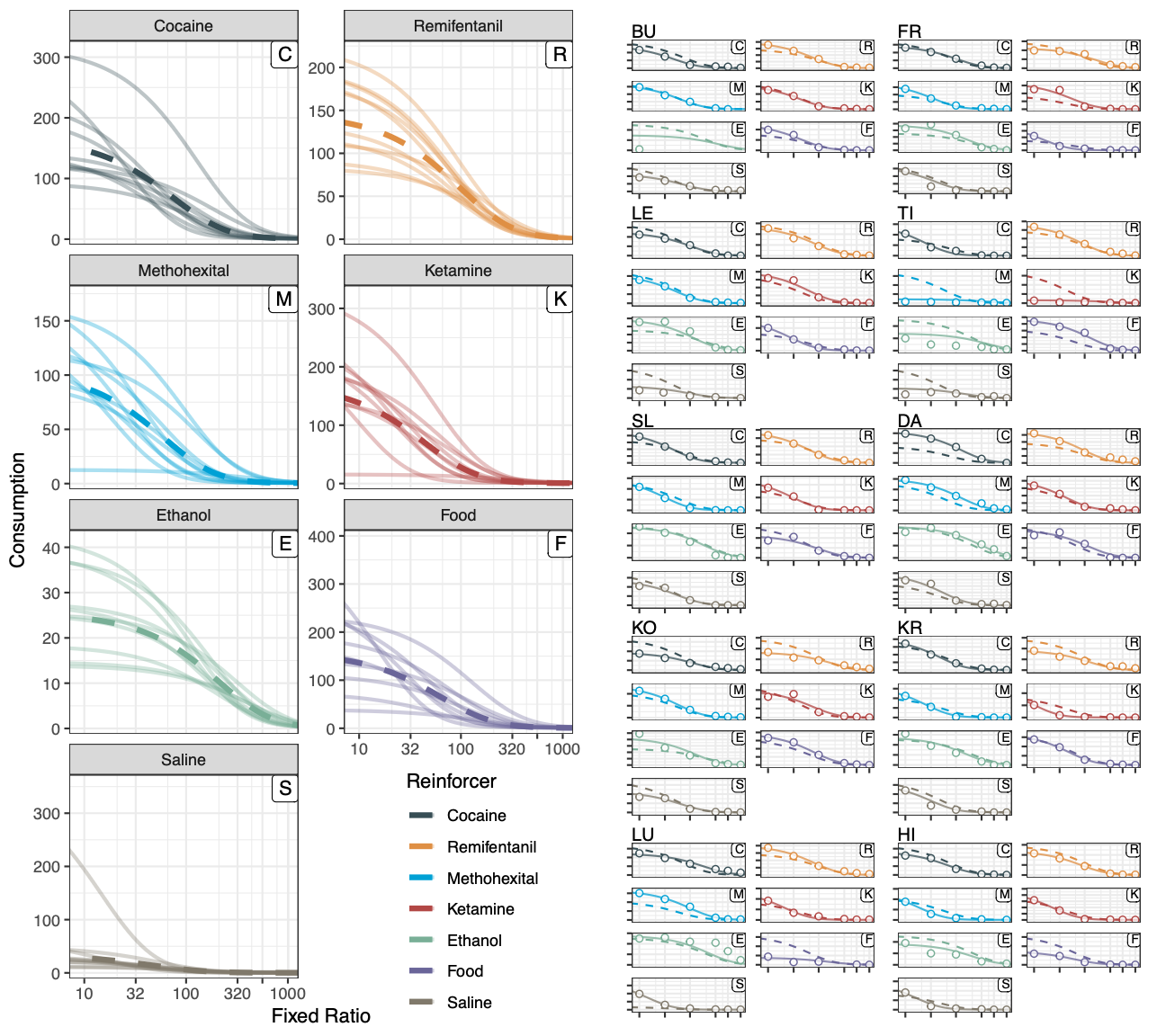
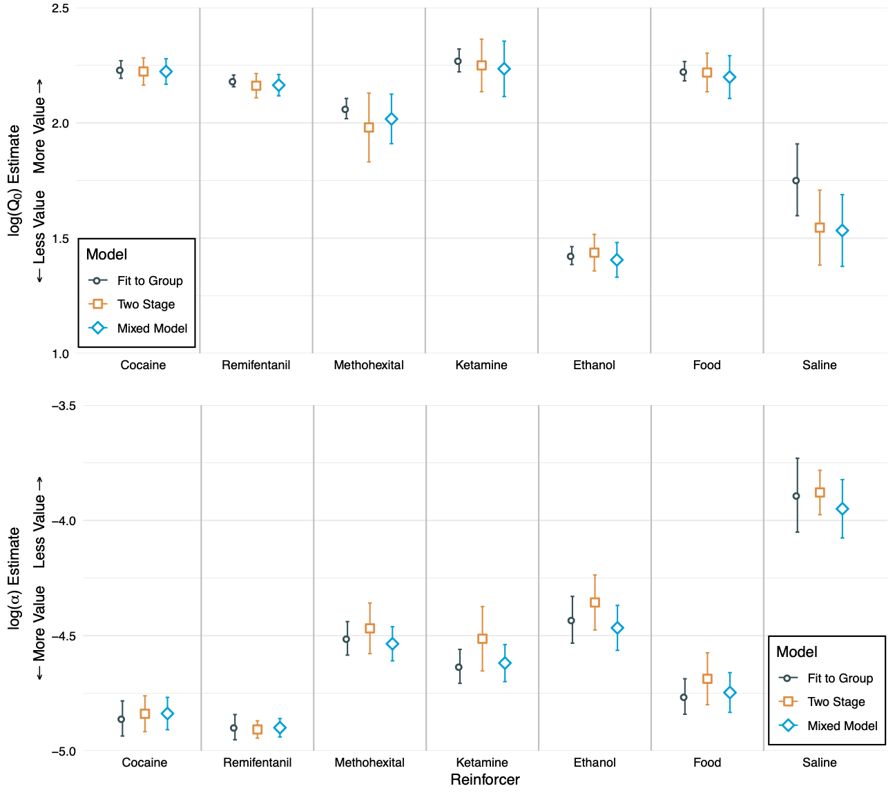
Applications: Behavioral Economic Demand

For more, see the full paper (also available at codedbx.com)

Applications: Delay Discounting

Delay discounting (how future rewards lose value relative to immediate ones) is often studied by fitting nonlinear models (hyperbolic, hyperboloid, exponential) for each person. Historically, researchers would drop participants with non-systematic data (e.g., inconsistent choices) to compute average discount rates.
Mixed-effects models offer a better solution: include random effects for individual discounting parameters instead of dropping data. This way, even “noisy” participants inform the model, but they are not allowed to distort the overall estimate.
Real-world example: Kirkpatrick et al. (2018) examined delay discounting data where ~20% of participants had to be excluded under traditional criteria (non-systematic responders). They applied a mixed-effects regression instead, which accounted for those individuals’ shallow discounting slopes as random effects.
Result: The model showed that those “problematic” participants systematically differed (shallower discount curves), and removing them would have biased the results.
Takeaway: In delay discounting and similar analyses, mixed models help estimate population parameters (like group-level discount rates) while letting each individual have their own \(k\) parameter, improving generalizability and reducing data loss.

Special Considerations in Fitting Mixed Effects Models

Autocorrelation: SCED and behavioral economic data often have autocorrelation (each observation is correlated with its neighbors in time). Standard mixed models (like lmer) may not adequately account for this autocorrelation, so you may need to add a explicit autocorrelation structure. Look at autocorrelation/partial autocorrelation plots and model-based autoregressive terms.
Small N (few subjects): With very few subjects, a complex random-effects model might not be identifiable. For example, if you have only 3 subjects, a random slope model is risky. You might stick to random intercepts, or even treat subject as fixed if needed (though that forfeits generalization). In such cases, Bayesian methods (brms) with informative priors or partial pooling can still stabilize estimates.
Centering and scaling: In SCEDs, time is often coded as session number. For better interpretation, you might center time at a meaningful point (e.g., session 0 at intervention start) so intercepts represent baseline level.
Phase changes: If you have phases (baseline vs treatment) per case, consider modeling phase as a fixed effect and perhaps allowing a random treatment effect (random slope on the treatment indicator) if cases might respond differently to treatment. This random treatment effect is akin to each case having its own intervention effect size.
Check model fit: With SCED data, use visual analyses… by plotting each individual’s fitted values vs. actual data to ensure the model is capturing the patterns.
Nonlinear models: Demand and discounting are inherently nonlinear. These models are sometimes hard to fit with conventional techniques, and sometimes much harder with mixed-effects models.

Special Considerations in Fitting Mixed Effects Models

“Nonsystematic” responses: As mentioned, some participants give data that don’t follow the typical curve shape (e.g., increasing demand when price is high, or erratic discounting). Instead of excluding them, mixed models include them with perhaps a larger residual or a random effect that captures their idiosyncrasy. This way, the group estimates aren’t skewed but those individuals are still represented (with higher uncertainty for their estimates).
Between-subject factors: In demand studies, you might have group comparisons (e.g., clinical vs. control group). Mixed models can incorporate this by adding a fixed effect for group and even allowing interactions (maybe the two groups have different average demand curves) while still having random subject effects. This is more elegant than analyzing groups separately.
Interpretation caution: With random effects on nonlinear parameters, interpretation is a bit trickier (e.g., the mean of a random \(k\) on a log-scale might be reported). But the payoff is often times worth it.

Key Takeaways

Mixed-effects models = fixed + random: They let us model overall effects of predictors (fixed) while accounting for variability across subjects or other units (random).
Retain individual information: Unlike averaging, conventional statistical techniques like t-tests, or fixed effects only models, mixed models don’t wash out individual differences. Each subject can have their own intercept, slope, etc., which improves accuracy and often ecological validity of findings.
Ideal for nested data: Whenever you have observations grouped by individual, clinic, classroom, etc., or repeated measures per subject, consider a mixed model. It will typically yield more appropriate inferences (e.g., correct standard errors) than treating all data as independent.
Behavior analysis fit: Mixed models address the concerns of behavior analysts by bridging group summary and single-case focus. You can get population-level insight and respect uniqueness of each case.
Use the right tools: Start simple (random intercepts) and only complexity if needed (random slopes, etc.). Check model diagnostics and don’t ignore warnings.

Further Resources

R packages

lme4
nlme
glmmTMB
multilevel
brms
beezdemand

scdhlm
The scdhlm package PDF (Hedges et al.) includes multiple examples of analyzing single-case data (e.g., Laski dataset) and is a great resource for SCED researchers (scdhlm: Estimating Hierarchical Linear Models for Single-Case Designs).

Further Resources

Books & Chapters & Papers:

Young, M. E. (2017). Discounting: A practical guide to multilevel analysis of indifference data. Journal of the Experimental Analysis of Behavior, 108(1), 97-112.
Young, M. E. (2018). Discounting: A practical guide to multilevel analysis of choice data. Journal of the Experimental Analysis of Behavior, 109(2), 293-312.
For an accessible start, see Chapter 16: Multilevel Modeling in Discovering Statistics Using R by Field et al., or Gelman & Hill (2007) for a comprehensive but readable text on multilevel models (with examples in R).
McElreath (2020), Statistical Rethinking: A Bayesian Course with Examples in R and Stan. This is a fantastic resource focused on the intuition behind a Bayesian approach that intertwines fundamental concepts of mixed models. As a plus, he posts videos on YouTube.

Online Tutorials:

The UCLA IDRE website’s guide “Introduction to Linear Mixed Models” (Introduction to Linear Mixed Models - OARC Stats - UCLA) is a practical walkthrough.
The University of Bristol’s Centre for Multilevel Modeling offers free online course materials and tutorials (with examples in R).

Further Resources

R Packages Documentation:

The lme4 vignette “Models of Mathematic Achievements” and the brms vignettes contain step-by-step examples. The scdhlm package PDF (Hedges et al.) includes multiple examples of analyzing single-case data (e.g., Laski dataset) and is a great resource for SCED researchers.

Practice:

Finally, nothing beats practicing on real data. Try re-analyzing a simple published single-case study with a mixed model or simulate a small dataset to see how mixed models work.
I make alot of my work available on my GitHub, including code and data.

Thank You

Brent Kaplan, PhD | codedbx.com | github.com/brentkaplan

Visit my website or email me at bkaplan.ku@gmail.com

Questions?