Bayesian discounting models with brms • beezdiscounting

The Bayesian tier fits the same discounting models as fit_dd_tmb() and fit_dd_choice(mode = "structural") using brms and Stan, with the discount rate estimated on the same natural-log scale. The fits below are precomputed (Stan sampling takes minutes), so the outputs shown come from real fits; copy the chunks into your session to reproduce them. brms, posterior, and loo are suggested packages.

Indifference points

data(dd_ip)

fit <- fit_dd_brms(
  dd_ip,
  equation = "mazur",
  family = "beta",
  boundary = "squeeze",   # dd_ip has exact 0/1 responses; see below
  chains = 4, cores = 4, seed = 1
)

summary(fit)
#> 
#> Bayesian Mixed-Effects Discounting Model Summary (brms)
#> ================================================== 
#> 
#> Equation: mazur  Family: beta 
#> Backend: brms 
#> Converged: Yes 
#> Subjects: 100  Observations: 600 
#> Diagnostics: rhat_max = 1.005, divergences = 0, min bulk ESS = 559
#> 
#> Coefficients (posterior median / SD, natural scale):
#>   term_display estimate std.error
#>  k:(Intercept)    0.325   0.03308
#> 
#> Variance components:
#>                Component Estimate   Scale
#>  sigma_u (log10-k RE SD)   0.4286   log10
#>          phi (precision)  28.5854 natural
tidy(fit)        # k on the natural scale (posterior medians of exp draws)
#> # A tibble: 3 × 8
#>   term             estimate std.error statistic p.value component estimate_scale
#>   <chr>               <dbl>     <dbl>     <dbl>   <dbl> <chr>     <chr>         
#> 1 k:(Intercept)       0.325    0.0331        NA      NA fixed     natural       
#> 2 sigma_u (log10-…    0.429   NA             NA      NA variance  log10         
#> 3 phi (precision)    28.6     NA             NA      NA variance  natural       
#> # ℹ 1 more variable: term_display <chr>
confint(fit)     # equal-tailed credible intervals
#> # A tibble: 1 × 5
#>   term          estimate conf.low conf.high level
#>   <chr>            <dbl>    <dbl>     <dbl> <dbl>
#> 1 k:(Intercept)    0.325    0.267     0.395  0.95
head(ranef(fit)) # per-subject log k offsets (ln scale) and k
#>     id     r_logk         k
#> 1   P1 -0.1571624 0.2758678
#> 2  P10  0.9286493 0.8219529
#> 3 P100  0.4245741 0.4981406
#> 4  P11  0.2369896 0.4114677
#> 5  P12 -0.5699986 0.1839221
#> 6  P13  0.6143202 0.5950892

The posterior discount curve is what the Bayesian fit adds over a point estimate. plot() draws the population curve (random effects set to zero) with an equal-tailed credible band for the conditional mean, over the observed (boundary-squeezed) indifference points; type = "parameters" shows each subject’s posterior k with its credible interval.

plot(fit, type = "population")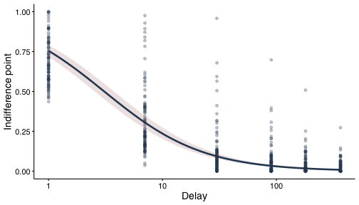

Posterior population discount curve with a 95% credible band over the observed indifference points.

plot of chunk post-curve

plot(fit, type = "parameters")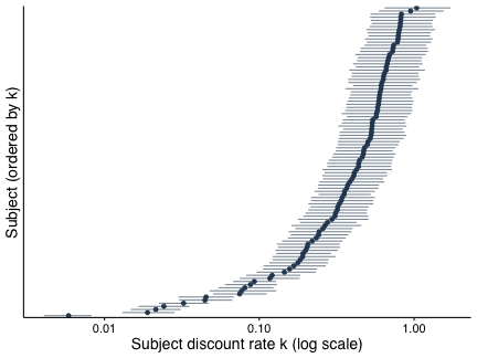

Posterior subject-level discount rates, each with a 95% credible interval, on a log scale.

plot of chunk post-k

Families and boundaries

The TMB tier’s SLT-beta family has no brms equivalent. Two options cover the same ground:

family = "beta" (default): brms’s beta likelihood with an identity link; the mean function is squished into (1e-6, 1 - 1e-6), mirroring the TMB mean clamp. The beta likelihood is not the SLT-beta: it cannot evaluate responses at exactly 0 or 1, so its estimates are not expected to match fit_dd_tmb(family = "sltb") when responses sit at or near the boundaries. Boundary responses are handled by boundary, which must be chosen explicitly when any are present: the default "error" refuses to fit and reports the count; "squeeze" applies the Smithson-Verkuilen transform (y(N-1) + 0.5)/N to every response, which floors the response at 0.5/N and can pull k downward when the fitted curve approaches that floor (long delays, steep discounting); "zoib" switches to a zero-one-inflated beta – more explicit about boundary responding, but it changes the estimand: k then describes the interior responses only. summary() reports the fraction of exact- and near-boundary responses.
family = "gaussian": matches fit_dd_tmb(family = "gaussian") wherever the TMB mean clamp (into [1e-6, 1 - 1e-6]) does not bind, i.e., everywhere except extreme decay underflow. In our validation harness the posterior median of log k lands within hundredths of the TMB MLE.

Priors

k is delay-unit dependent (per-day vs per-week k differ by a factor of 7), so the default logk prior anchors to the data: it centers k * median(delay) = 1, the delay at which the Mazur curve crosses one half. The anchor is printed at fit time, stored in fit$autoscale_info, and the whole table is inspectable and overridable:

default_dd_priors("mazur", family = "beta", data = dd_ip)
#>                  prior class      coef group resp dpar nlpar   lb   ub source
#>  normal(-4.09434, 2.5)     b Intercept                  logk <NA> <NA>   user
#>     student_t(3, 0, 1)    sd                            logk <NA> <NA>   user
#>          gamma(2, 0.1)   phi                                 <NA> <NA>   user

Override any row by passing a brms::set_prior() (shown here without re-fitting):

fit2 <- fit_dd_brms(
  dd_ip,
  equation = "mazur",
  boundary = "squeeze",
  prior = brms::set_prior("normal(-3, 1)", class = "b",
                          coef = "Intercept", nlpar = "logk")
)

The two-parameter equations ("green-myerson", "rachlin") add a population-level shape exponent with prior normal(0, 0.5) on log s (s near 1 a priori, 95% of the prior mass on roughly 0.38–2.66); zero delays are valid for Rachlin (the implementation guards the 0^s case exactly as the TMB template does).

These defaults are weakly regularising, not uninformative. With few subjects, the log s prior pulls the k–s pair of the two-parameter equations toward s = 1 (the pair is poorly identified from indifference points alone), and the half-t priors on the random-effect SDs matter when there are about 30 subjects or fewer. Report a prior-sensitivity check (refit with wider logk/logs priors) alongside two-parameter fits.

Rachlin needs one more step. Changing the delay unit by a factor c rescales Rachlin’s k by c^s, not c, so a prior centre in data units would describe a different curve prior in days than in weeks whenever s is not 1. fit_dd_brms() therefore samples Rachlin on the normalised delay x / median(x) (stored as fit$param_info$delay_scale), where the logk intercept prior is normal(0, 2.5), and converts the draws back to data-unit k before reporting. The same data in days or in weeks then gives the same curve posterior. A custom Rachlin logk intercept prior is read on the normalised scale, and the raw draws in fit$brmsfit are normalised; use coef(), confint() and get_dd_param_emms() for data-unit k.

Trial-level choice

ctrl <- simulate_dd_choice(n_subjects = 12, log_k_pop = log(0.01), seed = 7)
trt <- simulate_dd_choice(n_subjects = 12, log_k_pop = log(0.04), seed = 8)
trt$id <- paste0("t", trt$id)
ctrl$group <- "ctrl"
trt$group <- "treat"
choice_data <- rbind(ctrl, trt)

fitc <- fit_dd_choice_brms(
  choice_data,
  equation = "mazur",
  chains = 4, cores = 4, seed = 1
)

tidy(fitc)              # k and gamma (choice sensitivity), natural scale
#> # A tibble: 3 × 8
#>   term             estimate std.error statistic p.value component estimate_scale
#>   <chr>               <dbl>     <dbl>     <dbl>   <dbl> <chr>     <chr>         
#> 1 k:(Intercept)      0.0202   0.00420        NA      NA fixed     natural       
#> 2 gamma              3.61     0.579          NA      NA shape     natural       
#> 3 sigma_u (log10-…   0.240   NA              NA      NA variance  log10         
#> # ℹ 1 more variable: term_display <chr>
head(predict(fitc))     # P(choosing the larger-later), with intervals
#> # A tibble: 6 × 9
#>   id    ss_amount ll_amount delay choice   rel .fitted .lower .upper
#>   <fct>     <dbl>     <dbl> <dbl>  <dbl> <dbl>   <dbl>  <dbl>  <dbl>
#> 1 1            40        65    25      1  1.62  0.619  0.343   0.848
#> 2 1            55        75    61      0  1.36  0.239  0.0890  0.530
#> 3 1            31        85    14      1  2.74  0.987  0.925   0.999
#> 4 1            14        25    19      1  1.79  0.774  0.526   0.927
#> 5 1            47        60   160      1  1.28  0.0906 0.0313  0.251
#> 6 1            25        30     7      0  1.2   0.562  0.448   0.653

The structural likelihood is identical to fit_dd_choice(mode = "structural"): logit P(LL) = [b0] + gamma ((ll/ss) D(k, delay) - 1). The descriptive (Young 2018) mode is not wrapped; it is a plain logistic GLMM you can fit directly with brms::brm() if you want it Bayesian.

Between-subject designs on log k work as in fit_dd_choice() (gamma and b0 stay population-level), and the draws-based EMM/comparison helpers accept the result:

fitc_grp <- fit_dd_choice_brms(
  choice_data,
  equation = "mazur",
  factors = "group",
  chains = 4, cores = 4, seed = 1
)

get_dd_param_emms(fitc_grp)      # marginal k per group
#> # A tibble: 2 × 6
#>   level            k k_log std.error conf.low conf.high
#>   <chr>        <dbl> <dbl>     <dbl>    <dbl>     <dbl>
#> 1 group=ctrl  0.0120 -4.43     0.248  0.00742    0.0194
#> 2 group=treat 0.0343 -3.37     0.235  0.0212     0.0531
get_dd_comparisons(fitc_grp)     # log10 contrasts + ratios, post.prob
#> $k
#> $k$emmeans
#> # A tibble: 2 × 6
#>   level            k k_log std.error conf.low conf.high
#>   <chr>        <dbl> <dbl>     <dbl>    <dbl>     <dbl>
#> 1 group=ctrl  0.0120 -4.43     0.248  0.00742    0.0194
#> 2 group=treat 0.0343 -3.37     0.235  0.0212     0.0531
#> 
#> $k$contrasts_log10
#> # A tibble: 1 × 9
#>   contrast         estimate std.error statistic    df conf.low conf.high p.value
#>   <chr>               <dbl>     <dbl>     <dbl> <dbl>    <dbl>     <dbl>   <dbl>
#> 1 group=ctrl - gr…   -0.451     0.142        NA    NA   -0.726    -0.168      NA
#> # ℹ 1 more variable: post.prob <dbl>
#> 
#> $k$contrasts_ratio
#> # A tibble: 1 × 6
#>   contrast                 ratio conf.low conf.high p.value post.prob
#>   <chr>                    <dbl>    <dbl>     <dbl>   <dbl>     <dbl>
#> 1 group=ctrl - group=treat 0.354    0.188     0.679      NA     0.999
#> 
#> 
#> attr(,"class")
#> [1] "beezdiscounting_comparison"
#> attr(,"backend")
#> [1] "brms"
#> attr(,"adjustment_method")
#> [1] "none (posterior summaries; see post.prob)"
#> attr(,"compare_specs_used")
#> [1] "all fitted factors"
#> attr(,"contrast_type_used")
#> [1] "pairwise"
#> attr(,"contrast_by_used")
#> [1] "NULL"

Reading Bayesian output

tidy() keeps the package’s exact eight-column contract, with statistic/p.value set to NA: estimates are posterior medians of the report-space-transformed draws (no delta method), and intervals live in confint().
glance() reports elpd_loo/looic plus R-hat/ESS/divergence diagnostics; logLik/AIC/BIC are NA by design. Compare Bayesian fits with brms::loo_compare(fit$brmsfit, fit2$brmsfit).
fit$converged requires R-hat < 1.01, zero divergences, and bulk ESS >= 400; components are in fit$mcmc_info, and the full brms toolbox is available on fit$brmsfit.

v1 scope

Random effects are an intercept on log k (k ~ 1), optionally with a per-subject precision intercept (k + phi ~ 1, beta family), as in the TMB tier. Two differences from the TMB tier remain: the TMB SLT-beta fit bounds the precision below at phi = 0.1 while the brms beta fit does not, and ranef() returns each subject’s log k offset on the natural-log scale, whereas ranef() on a one-random-effect TMB fit returns the standardised deviate u. get_dd_param_emms() and get_dd_comparisons() accept Bayesian indifference-point and structural choice fits (quantile credible intervals; post.prob in place of adjusted p-values). Both Bayesian fitters support between-subject designs on log k via factors/factor_interaction/continuous_covariates, mirroring their TMB counterparts.