Getting started: indifference points, k, and AUC

This vignette covers the everyday delay-discounting workflow in beezdiscounting: screen the data for quality, fit a discounting model to get a rate k, and compute area under the curve (AUC) as a model-free summary. It is the place to start before moving on to the mixed-effects and Bayesian tiers.

Indifference points

A delay-discounting task trades a smaller-sooner reward against a larger-later one across several delays. At each delay the indifference point is the immediate amount that feels equivalent to the later reward, expressed as a proportion of that later reward, which places it on [0, 1]. A value near 1 means the person barely discounts the delay; a value near 0 means the delayed reward is worth almost nothing to them.

beezdiscounting works with long-format data: one row per subject per delay, with columns id, x (the delay), and y (the indifference point). Here is one well-behaved subject:

clean <- data.frame(
  id = "demo",
  x  = c(1, 7, 30, 90, 180, 365),
  y  = c(0.95, 0.81, 0.55, 0.32, 0.17, 0.08)
)
clean
#>     id   x    y
#> 1 demo   1 0.95
#> 2 demo   7 0.81
#> 3 demo  30 0.55
#> 4 demo  90 0.32
#> 5 demo 180 0.17
#> 6 demo 365 0.08

Screening for unsystematic data

Before fitting anything, check whether each subject’s indifference points form an orderly, decreasing pattern. check_unsystematic() applies the two criteria of Johnson and Bickel (2008) to each subject’s points, taken in delay order, and returns one row per id:

check_unsystematic(clean)
#> # A tibble: 1 × 3
#>   id    c1_pass c2_pass
#>   <chr> <lgl>   <lgl>  
#> 1 demo  TRUE    TRUE

Criterion 1 (c1_pass) flags non-systematic increases: no indifference point may exceed the immediately preceding (shorter-delay) point by more than c1 (default 0.2, i.e. 20% of the larger reward).
Criterion 2 (c2_pass) flags a lack of overall discounting: the last indifference point must fall at least c2 (default 0.1) below the first.

Our demo subject passes both. Treat a failure as a signal to inspect that subject’s data rather than as an automatic exclusion. Noisy titration, a misunderstanding of the task, or genuinely shallow discounting can all trip these rules.

Fitting a discounting model

fit_dd() fits either Mazur’s (1987) hyperbola, y = 1 / (1 + k * x), or the exponential model, y = exp(-k * x). The method argument controls how subjects are pooled: "two stage" fits each subject separately, "mean" fits the averaged indifference points, and "pooled" fits all rows together. results_dd() tidies the fitted object into a data frame of estimates and fit statistics:

fit <- fit_dd(clean, equation = "mazur", method = "two stage")
results_dd(fit)
#> # A tibble: 1 × 22
#>   method  id    term  estimate std.error statistic p.value  sigma isConv  finTol
#>   <chr>   <chr> <chr>    <dbl>     <dbl>     <dbl>   <dbl>  <dbl> <lgl>    <dbl>
#> 1 two st… demo  k       0.0271   0.00157      17.3 1.18e-5 0.0223 TRUE   1.49e-8
#> # ℹ 12 more variables: logLik <dbl>, AIC <dbl>, BIC <dbl>, deviance <dbl>,
#> #   df.residual <int>, nobs <int>, R2 <dbl>, auc_regular <dbl>,
#> #   auc_log10 <dbl>, auc_ord <dbl>, conf_low <dbl>, conf_high <dbl>

The estimate column is k, the discount rate: larger values mean steeper discounting. results_dd() also returns the standard error, a confidence interval (conf_low, conf_high), R2, and the usual information criteria. Swap equation = "exponential" to fit and compare the exponential form.

Plot the fit against the observed points with plot_dd():

plot_dd(fit)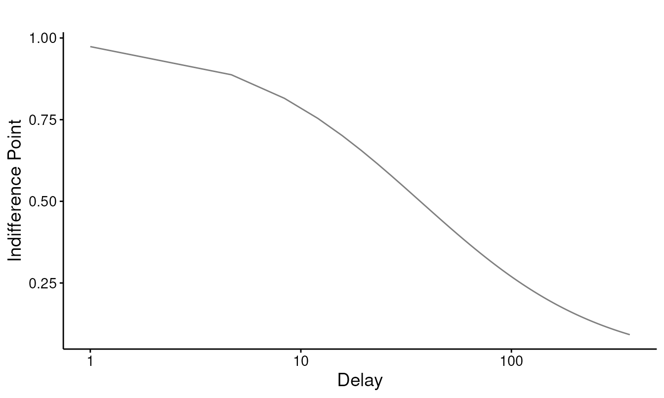

Area under the curve

AUC (Myerson, Green & Warusawitharana, 2001) summarizes discounting without committing to a model: the normalized area beneath the indifference points, running from 1 (no discounting) toward 0 (steep discounting). calc_aucs() returns three variants:

calc_aucs(clean)
#> # A tibble: 1 × 4
#>   id    auc_regular auc_log10 auc_ord
#>   <chr>       <dbl>     <dbl>   <dbl>
#> 1 demo        0.253     0.550   0.473

auc_regular integrates over the raw delays; auc_log10 and auc_ord integrate over log-spaced and ordinally-spaced delays, the rescalings recommended by Borges et al. (2016) so that closely-spaced short delays do not dominate the area. Like check_unsystematic(), calc_aucs() returns one row per subject. Use AUC when you want an atheoretical index, or alongside k as a robustness check.

Working at scale

The built-in dd_ip dataset has 100 simulated subjects measured at six delays:

data(dd_ip)
str(dd_ip)
#> 'data.frame':    600 obs. of  3 variables:
#>  $ id: chr  "P1" "P1" "P1" "P1" ...
#>  $ x : num  1 7 30 90 180 365 1 7 30 90 ...
#>  $ y : num  0.8163 0.3909 0.0192 0.0991 0.0135 ...
length(unique(dd_ip$id))
#> [1] 100

Fit every subject in one call and summarize the resulting rates:

fits <- fit_dd(dd_ip, equation = "mazur", method = "two stage")
res <- results_dd(fits)
summary(res$estimate)   # distribution of k across subjects
#>     Min.  1st Qu.   Median     Mean  3rd Qu.     Max. 
#> 0.005304 0.221916 0.503760 0.490939 0.724008 1.186899
summary(res$R2)         # per-subject fit
#>    Min. 1st Qu.  Median    Mean 3rd Qu.    Max. 
#>  0.8013  0.9678  0.9810  0.9729  0.9900  0.9984

The hyperbola fits these subjects well (median R2 around 0.98). A two-stage fit also returns each subject’s AUC, so the model-free indices come back in the same table:

head(res[c("id", "estimate", "auc_regular", "auc_log10", "auc_ord")])
#> # A tibble: 6 × 5
#>   id    estimate auc_regular auc_log10 auc_ord
#>   <chr>    <dbl>       <dbl>     <dbl>   <dbl>
#> 1 P1       0.248      0.0509     0.235  0.186 
#> 2 P10      0.907      0.0112     0.111  0.0838
#> 3 P100     0.544      0.0492     0.163  0.131 
#> 4 P11      0.480      0.0348     0.175  0.138 
#> 5 P12      0.193      0.0648     0.272  0.218 
#> 6 P13      0.697      0.0213     0.133  0.102

check_unsystematic() and calc_aucs() both take the whole data frame and return one row per subject, so screening the full sample is a single call:

screen <- check_unsystematic(dd_ip)
colMeans(screen[c("c1_pass", "c2_pass")])
#> c1_pass c2_pass 
#>       1       1

Every subject passes both criteria, which is what we expect from cleanly simulated data. With real data the proportion failing each criterion tells you how much of the sample shows orderly discounting before you commit to a model.

Where to go next

For multi-subject data, the mixed-effects tier estimates the population rate and subject-level rates jointly and handles indifference points that pile up at 0 and 1. See:

vignette("sltb-discounting") for why bounded indifference points need a bounded error distribution, and the SLT-beta mixed model.
vignette("tmb-mixed-effects") for the fit_dd_tmb() workflow and its methods.
vignette("dd-group-comparisons") for comparing discount rates between groups.
vignette("bayesian-discounting") for the Bayesian tier via brms.

References

Borges, A. M., Kuang, J., Milhorn, H., & Yi, R. (2016). An alternative approach to calculating area-under-the-curve (AUC) in delay discounting research. Journal of the Experimental Analysis of Behavior, 106, 145–155.
Johnson, M. W., & Bickel, W. K. (2008). An algorithm for identifying nonsystematic delay-discounting data. Experimental and Clinical Psychopharmacology, 16(3), 264–274.
Mazur, J. E. (1987). An adjusting procedure for studying delayed reinforcement. In The effect of delay and of intervening events on reinforcement value (pp. 55–73). Lawrence Erlbaum Associates.
Myerson, J., Green, L., & Warusawitharana, M. (2001). Area under the curve as a measure of discounting. Journal of the Experimental Analysis of Behavior, 76(2), 235–243.