The linearized Mazur hyperbola: closed-form k and an F-test for conditions

The other modeling tiers in beezdiscounting estimate the discount rate by optimization. fit_dd() fits Mazur’s hyperbola to each subject by nonlinear least squares, which may fail to converge for flat or erratic subjects, and fit_dd_tmb() fits a mixed model whose marginal likelihood has to be maximized numerically. Hinds et al. (2026) take a different route. They rearrange the hyperbola so that ln k appears as an intercept, at which point the per-subject estimate is a mean, the population model is a one-way random-effects ANOVA with closed-form maximum likelihood estimates, and condition means can be compared with an F-test whose null distribution holds at any sample size under the model’s assumptions. No optimizer is involved anywhere, so there is nothing to fail to converge. fit_dd_linear() implements that estimator.

This vignette covers (i) the transform and the per-subject estimator, (ii) the random-effects model and the methods that act on a fit, (iii) comparing conditions with the F-test, (iv) what to do with indifference points at exactly 0 or 1, and (v) how the linearized estimates relate to the nonlinear ones.

The transform

Mazur’s (1987) hyperbola gives the discounted value of a delayed reward as a proportion of its undelayed value, D = 1 / (1 + k t), where t is the delay and k is the discount rate. Solving for k and taking logs,

ln(1 / D - 1) - ln(t) = ln k .

Every indifference point, once transformed this way, is a direct read of ln k. Hinds et al. (2026) treat the transformed points as ln k plus additive Gaussian error, so the per-subject estimate of ln k is the mean of the transformed points (equivalently, the geometric mean of (1 / D - 1) / t). Note that the Gaussian error on the transformed scale is a modeling assumption, as it is for any other error model; Section 2 of the paper discusses it, and the last section below shows what it implies on the raw scale.

To make that concrete, here is one subject drawn from the simulator introduced in the next section, with the transform done by hand:

one <- simulate_dd_linear(1, delays = c(7, 30, 90, 180, 365, 730),
                          mu = c(demo = -6), sigma2 = 2, g = 10, seed = 3)
one$y_lin <- log(1 / one$y - 1) - log(one$x)
one
#>       id condition   x         y     y_lin
#> 1 demo_1      demo   7 0.9980227 -8.169936
#> 2 demo_1      demo  30 0.9818196 -7.390260
#> 3 demo_1      demo  90 0.9925035 -9.385603
#> 4 demo_1      demo 180 0.9077450 -7.479363
#> 5 demo_1      demo 365 0.8598136 -7.713640
#> 6 demo_1      demo 730 0.7393126 -7.635443
mean(one$y_lin)
#> [1] -7.962374

fit_dd_linear() returns the same number:

fit_dd_linear(one)$subjects[, c("id", "logk", "se", "ci_lo", "ci_hi")]
#> # A tibble: 1 × 5
#>   id      logk    se ci_lo ci_hi
#>   <chr>  <dbl> <dbl> <dbl> <dbl>
#> 1 demo_1 -7.96 0.305 -8.75 -7.18

The standard error and interval are the usual t-based quantities for a mean of T observations (here T = 6 delays), so for a given spread of transformed points a subject measured at more delays gets a narrower interval.

Simulate a three-condition study

simulate_dd_linear() draws data from the random-effects model that fit_dd_linear() fits: each subject’s ln k is drawn around their condition mean mu, and each transformed point is that subject’s ln k plus Gaussian noise. The model has two variance parameters. sigma2 is the noise variance on the transformed scale, and g scales the between-subject variance, Var(ln k_i) = g * sigma2 / T. The values below are of the order the paper reports for real data (sigma2 near 2, g near 10). A scalar n_subjects is recycled across conditions, so this call yields 30 subjects per condition and 90 in total. Conditions A and C share a mean; B discounts more steeply by 1.5 on the ln k scale (a factor of about 4.5 in k).

sim <- simulate_dd_linear(
  n_subjects = 30,
  delays     = c(7, 30, 90, 180, 365, 730),
  mu         = c(A = -6, B = -4.5, C = -6),
  sigma2     = 2,
  g          = 10,
  seed       = 1
)
head(sim)
#>    id condition   x         y
#> 1 A_1         A   7 0.9974397
#> 2 A_1         A  30 0.8843580
#> 3 A_1         A  90 0.7316237
#> 4 A_1         A 180 0.7232288
#> 5 A_1         A 365 0.2688872
#> 6 A_1         A 730 0.4405031

The layout is the package’s usual long format (id, x for delay, y for the indifference point on [0, 1]) plus the condition column.

Fit and inspect

factors names the one between-subject column that defines the conditions. Two design requirements apply to the random-effects part of the fit: every subject must appear under exactly one level (the F-test assumes independent units per condition), and every subject must contribute the same number of usable delays. A within-subject factor is rejected with an error; an unbalanced design (see the boundary section below) returns the per-subject estimates but leaves the population component unfitted.

fit <- fit_dd_linear(sim, factors = "condition")
fit
#> Linearized Mazur discounting fit (Hinds et al., 2026)
#>   90 units, 6 delays each, factor: condition
#>   boundary = "clamp" (eps = 0.005): 0 point(s) at 0/1, 0 clamped, 0 dropped
#>   Population ln k (mu):
#>      A      B      C 
#> -5.879 -4.232 -5.797 
#>   sigma2 = 2.145, g = 6.940, logLik(raw) = 382.04

The print method reports the design, the boundary bookkeeping (nothing to report here, as the simulator keeps every point strictly inside (0, 1)), the condition means mu on the ln k scale, and the two variance estimates. summary() adds the first rows of the per-subject table and the population parameters as a tibble:

summary(fit)
#> Linearized Mazur discounting fit (Hinds et al., 2026)
#>   90 units, 6 delays each, factor: condition
#>   boundary = "clamp" (eps = 0.005): 0 point(s) at 0/1, 0 clamped, 0 dropped
#>   Population ln k (mu):
#>      A      B      C 
#> -5.879 -4.232 -5.797 
#>   sigma2 = 2.145, g = 6.940, logLik(raw) = 382.04
#> 
#> Per-unit ln k (first 10):
#> # A tibble: 10 × 7
#>    id    condition  logk    se  ci_lo ci_hi n_boundary
#>    <chr> <fct>     <dbl> <dbl>  <dbl> <dbl>      <int>
#>  1 A_1   A         -6.04 0.431  -7.15 -4.94          0
#>  2 A_10  A         -7.19 0.788  -9.22 -5.17          0
#>  3 A_11  A         -4.04 0.419  -5.11 -2.96          0
#>  4 A_12  A         -5.04 0.676  -6.78 -3.30          0
#>  5 A_13  A         -6.70 0.761  -8.65 -4.74          0
#>  6 A_14  A         -9.37 0.533 -10.7  -8.00          0
#>  7 A_15  A         -2.83 0.505  -4.13 -1.53          0
#>  8 A_16  A         -6.35 0.564  -7.80 -4.90          0
#>  9 A_17  A         -6.13 0.512  -7.45 -4.81          0
#> 10 A_18  A         -4.69 0.653  -6.36 -3.01          0
#> 
#> Population parameters:
#> # A tibble: 5 × 2
#>   term   estimate
#>   <chr>     <dbl>
#> 1 mu_A      -5.88
#> 2 mu_B      -4.23
#> 3 mu_C      -5.80
#> 4 sigma2     2.14
#> 5 g          6.94

coef() returns the condition means and confint() an interval around each. The paper gives no population interval, so the package uses the ANOVA-style t-interval on the per-subject ln k values (between-subject mean square, N - C degrees of freedom); with parm = "subject" you get the per-subject intervals instead.

coef(fit)
#>         A         B         C 
#> -5.879258 -4.232474 -5.797496
confint(fit)
#>       2.5 %    97.5 %
#> A -6.501060 -5.257457
#> B -4.854276 -3.610672
#> C -6.419298 -5.175695
head(confint(fit, parm = "subject"), 3)
#>          2.5 %    97.5 %
#> A_1  -7.150000 -4.935422
#> A_10 -9.216172 -5.166594
#> A_11 -5.113410 -2.958965

tidy() returns the per-subject table by default (logk, its se and interval, k back-transformed with its interval, and n_boundary, the count of points that sat at 0 or 1), or the population parameters with effects = "population":

tidy(fit)
#> # A tibble: 90 × 15
#>    id    condition n_delays n_boundary  logk    se    df  ci_lo ci_hi         k
#>    <chr> <fct>        <int>      <int> <dbl> <dbl> <dbl>  <dbl> <dbl>     <dbl>
#>  1 A_1   A                6          0 -6.04 0.431     5  -7.15 -4.94 0.00238  
#>  2 A_10  A                6          0 -7.19 0.788     5  -9.22 -5.17 0.000753 
#>  3 A_11  A                6          0 -4.04 0.419     5  -5.11 -2.96 0.0177   
#>  4 A_12  A                6          0 -5.04 0.676     5  -6.78 -3.30 0.00647  
#>  5 A_13  A                6          0 -6.70 0.761     5  -8.65 -4.74 0.00123  
#>  6 A_14  A                6          0 -9.37 0.533     5 -10.7  -8.00 0.0000852
#>  7 A_15  A                6          0 -2.83 0.505     5  -4.13 -1.53 0.0589   
#>  8 A_16  A                6          0 -6.35 0.564     5  -7.80 -4.90 0.00175  
#>  9 A_17  A                6          0 -6.13 0.512     5  -7.45 -4.81 0.00217  
#> 10 A_18  A                6          0 -4.69 0.653     5  -6.36 -3.01 0.00923  
#> # ℹ 80 more rows
#> # ℹ 5 more variables: k_lo <dbl>, k_hi <dbl>, s2 <dbl>, loglik_y <dbl>,
#> #   loglik_raw <dbl>
tidy(fit, effects = "population")
#> # A tibble: 5 × 2
#>   term   estimate
#>   <chr>     <dbl>
#> 1 mu_A      -5.88
#> 2 mu_B      -4.23
#> 3 mu_C      -5.80
#> 4 sigma2     2.14
#> 5 g          6.94

Because the data were simulated, the estimates can be set beside the values that generated them:

tibble::tibble(
  term     = c("mu_A", "mu_B", "mu_C", "sigma2", "g"),
  truth    = c(-6, -4.5, -6, 2, 10),
  estimate = tidy(fit, effects = "population")$estimate
)
#> # A tibble: 5 × 3
#>   term   truth estimate
#>   <chr>  <dbl>    <dbl>
#> 1 mu_A    -6      -5.88
#> 2 mu_B    -4.5    -4.23
#> 3 mu_C    -6      -5.80
#> 4 sigma2   2       2.14
#> 5 g       10       6.94

The means and sigma2 are recovered closely; g is estimated with more uncertainty, as a between-subject variance from 30 subjects per condition would be under any estimator.

glance() gives the one-row model summary used across the package for stacking fits (nobs() returns the count of usable transformed points, 540 here), and logLik() the log-likelihood. By default logLik() returns the population (random-effects) likelihood on the raw indifference-point scale, that is, corrected by the Jacobian of the transform (paper Section 2.3), which is what makes it comparable with the Gaussian likelihoods of fit_dd() and fit_dd_tmb(). scale = "transformed" returns the likelihood of the transformed points, and level = "subject" the sum of the per-subject likelihoods (the quantity to set against a per-subject fit rather than a mixed model).

glance(fit)
#> # A tibble: 1 × 12
#>   model_class     backend equation  nobs n_units n_conditions n_par sigma2     g
#>   <chr>           <chr>   <chr>    <int>   <int>        <int> <int>  <dbl> <dbl>
#> 1 beezdiscountin… closed… mazur_l…   540      90            3     5   2.14  6.94
#> # ℹ 3 more variables: logLik <dbl>, AIC <dbl>, BIC <dbl>
logLik(fit)
#> 'log Lik.' 382.0447 (df=5)

augment() returns the long data with the transformed value y_lin, the value actually used after boundary handling d_used, the fitted indifference point and residual on the raw scale, .fitted and .resid, and the standardized residual on the transformed scale, .std_resid (the residual divided by the model’s error standard deviation, sqrt(sigma2)). Together with tidy(), coef() and confint(), this table is what you need to reproduce or customize the figures that plot() draws in the Figures section.

head(augment(fit), 3)
#> # A tibble: 3 × 11
#>   id        x     y condition unit  y_lin d_used log_jac .fitted  .resid
#>   <chr> <dbl> <dbl> <fct>     <fct> <dbl>  <dbl>   <dbl>   <dbl>   <dbl>
#> 1 A_1       7 0.997 A         A_1   -7.91  0.997    5.97   0.984  0.0138
#> 2 A_1      30 0.884 A         A_1   -5.44  0.884    2.28   0.933 -0.0491
#> 3 A_1      90 0.732 A         A_1   -5.50  0.732    1.63   0.824 -0.0923
#> # ℹ 1 more variable: .std_resid <dbl>

Comparing conditions

anova() tests whether the condition means are equal. The statistic is the paper’s F (Proposition 3.5) with C - 1 and N - C degrees of freedom (here 2 and 87). Under the model’s assumptions (a balanced design, independent subjects, and Gaussian error on the transformed scale) its null distribution is F at any N, with no large-sample approximation involved. The proposition derives this for a positive between-subject variance estimate g, which is the usual case; when g is estimated at 0 the package still reports the statistic but warns.

anova(fit)
#> # A tibble: 1 × 6
#>   hypothesis     F   df1   df2  p_value cohens_d
#>   <chr>      <dbl> <int> <dbl>    <dbl>    <dbl>
#> 1 A = B = C   8.80     2    87 0.000331       NA

A hypothesis argument restricts the null to a subset of levels. To test only whether A and C share a mean (the two conditions the simulation set equal):

anova(fit, hypothesis = list(c("A", "C")))
#> # A tibble: 1 × 6
#>   hypothesis      F   df1   df2 p_value cohens_d
#>   <chr>       <dbl> <int> <dbl>   <dbl>    <dbl>
#> 1 A = C      0.0342     1    87   0.854  -0.0485

pairwise = TRUE runs every two-level comparison. The p-values are uncorrected, and each row also reports Cohen’s d on the ln k scale (the mean difference divided by the between-subject standard deviation); cohens_d is only defined for two-level hypotheses, which is why the overall test above shows NA.

anova(fit, pairwise = TRUE)
#> # A tibble: 3 × 6
#>   hypothesis       F   df1   df2  p_value cohens_d
#>   <chr>        <dbl> <int> <dbl>    <dbl>    <dbl>
#> 1 A = B      13.9        1    87 0.000350  -0.977 
#> 2 A = C       0.0342     1    87 0.854     -0.0485
#> 3 B = C      12.5        1    87 0.000651   0.929

B differs from both A and C at about one between-subject standard deviation, and A and C do not differ, which is the structure the simulation built in. By contrast, the Wald tests in vignette("dd-group-comparisons") rely on a large-sample approximation to the sampling distribution. The F-test here needs no such approximation, and it costs nothing beyond the closed-form fit.

Indifference points at 0 or 1

The transform is undefined at D = 0 and D = 1 (ln(1 / D - 1) diverges), and the paper does not address such values. Real titration data contain them. The package’s dd_ip dataset has 600 points from 100 subjects, of which 125 are exactly 0 and 4 lie above 1 (the input check clamps those to 1, with a warning), so 129 points sit on the boundary. boundary selects one of three policies.

"clamp" (the default) moves an exact 0 to eps and an exact 1 to 1 - eps. Only exact 0 and 1 are touched; an interior point, however close to a bound, is used as observed. The print method reports how many points were clamped.

data(dd_ip)
fit_clamp <- fit_dd_linear(dd_ip)
#> Warning: Clamped out-of-range y to [0, 1]: 4 value(s) > 1 set to 1, 0 value(s)
#> < 0 set to 0.
fit_clamp
#> Linearized Mazur discounting fit (Hinds et al., 2026)
#>   100 units, 6 delays each
#>   boundary = "clamp" (eps = 0.005): 129 point(s) at 0/1, 129 clamped, 0 dropped
#>   Population ln k (mu):
#>  (all) 
#> -1.077 
#>   sigma2 = 1.090, g = 4.901, logLik(raw) = 932.52

"drop" removes boundary points. The per-subject estimates are still returned, but subjects then differ in their number of usable delays, the design is no longer balanced, and the random-effects component is unavailable. The population methods (coef(), anova(), and the default confint(), tidy(effects = "population") and logLik()) then error; the per-subject versions still work.

fit_drop <- fit_dd_linear(dd_ip, boundary = "drop")
#> Warning: Clamped out-of-range y to [0, 1]: 4 value(s) > 1 set to 1, 0 value(s)
#> < 0 set to 0.
#> Warning: Random-effects component not fitted: design is not balanced after boundary
#> handling.
#> ℹ Per-unit estimates are still returned. `anova()` is unavailable.
fit_drop
#> Linearized Mazur discounting fit (Hinds et al., 2026)
#>   100 units, NA delays each
#>   boundary = "drop" (eps = 0.005): 129 point(s) at 0/1, 0 clamped, 129 dropped
#>   Random-effects component: not fitted (unbalanced design)

"error" refuses the data, which is the right choice in a pipeline that should never silently impute:

fit_dd_linear(dd_ip, boundary = "error")
#> Warning: Clamped out-of-range y to [0, 1]: 4 value(s) > 1 set to 1, 0 value(s)
#> < 0 set to 0.
#> Error in `.dd_lin_transform()`:
#> ! 129 indifference points equal 0 or 1; the linearized transform is
#>   undefined there.
#> ℹ Use `boundary = "clamp"` (default) or `"drop"`, or pre-process the data.

With a fifth of the points clamped, the population estimate depends on where the clamped points are placed. The default eps is 0.005; when ll (the larger-later amount) is supplied it becomes 1 / (2 * ll), half the smallest step the task could resolve. The table below refits dd_ip across a range of eps:

eps_grid <- c(0.001, 0.005, 0.01, 0.05)
tibble::tibble(
  eps = eps_grid,
  mu  = sapply(eps_grid, function(e) coef(fit_dd_linear(dd_ip, eps = e))),
  k   = exp(mu)
)
#> # A tibble: 4 × 3
#>     eps     mu     k
#>   <dbl>  <dbl> <dbl>
#> 1 0.001 -0.751 0.472
#> 2 0.005 -1.08  0.341
#> 3 0.01  -1.22  0.296
#> 4 0.05  -1.55  0.212

The estimate of ln k moves by 0.8 across this range, which is a factor of about 2.2 in k. The sensitivity arises when data with many points on the boundary meet a transform that diverges there and a clamp policy that has to pick a finite stand-in. A bounded likelihood needs no eps at all. We recommend setting eps from the task’s resolution via ll, reporting the clamped count, and, when boundary points are this common, preferring a likelihood that treats them as data; see vignette("sltb-discounting").

Figures

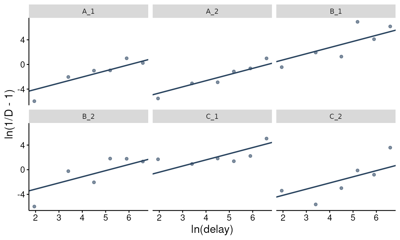
plot() draws the pictures that go with the fit and shares its core arguments (type, ids, n_points, x_trans, show_observed) with the other indifference-point tiers. The linearization is easiest to see on the transformed scale. For each subject, ln(1 / D - 1) plotted against ln(t) should scatter around a line of slope 1 whose intercept is that subject’s ln k. type = "transformed" draws that picture, one panel per subject; ids picks the subjects (without it, the first twelve are shown):

show <- c("A_1", "A_2", "B_1", "B_2", "C_1", "C_2")
plot(fit, type = "transformed", ids = show)

Six panels, one per simulated subject, plotting ln(1/D - 1) against ln(delay); the points in each panel scatter around a line of slope 1 whose intercept is the subject's estimated ln k.

Back on the raw scale, plot(fit) draws the hyperbola implied by each condition’s geometric-mean k, exp(mu), over the observed indifference points. type = "individual" adds each subject’s own hyperbola, 1 / (1 + k x), underneath (here for the same six subjects):

plot(fit, type = "individual", ids = show)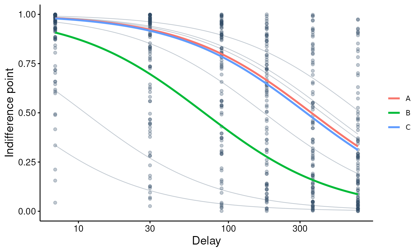

Observed indifference points against delay on a log axis, with three coloured condition curves and six thin per-subject hyperbolae drawn underneath them.

The third figure answers the study question. type = "parameters" shows every subject’s ln k with its t-interval, by condition, with the condition mean and its interval (the values from coef() and confint()) overlaid. The axis is ln k, the scale on which the model is fitted and its effect size is defined; k_scale = "log10" draws the same picture as k on a log axis, the convention of the other tiers.

plot(fit, type = "parameters")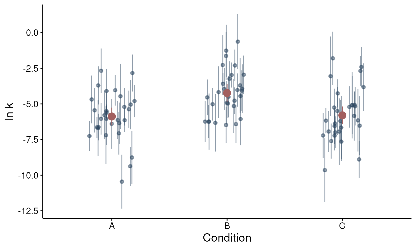

Per-subject ln k estimates with confidence intervals, jittered within three conditions A, B, and C; condition B sits about 1.5 units higher than A and C, and the condition means with their intervals are overlaid in a contrasting colour.

The frames behind these figures come from augment(), tidy(), coef() and confint(), for anyone who wants a different picture.

How this relates to the nonlinear fit

The same data fitted subject by subject with fit_dd() give a second set of per-subject rates. The two estimators target the same k under different error models: fit_dd() assumes Gaussian error on the indifference-point scale, whereas fit_dd_linear() assumes it on the transformed scale, where a fixed error in ln(1 / D - 1) corresponds to a small raw-scale error near D = 0.5 and a much smaller one near the bounds.

nls_fit <- fit_dd(sim, equation = "mazur", method = "two stage")
nls_res <- results_dd(nls_fit)
both <- merge(
  tidy(fit)[, c("id", "condition", "logk")],
  data.frame(id = nls_res$id, logk_nls = log(nls_res$estimate)),
  by = "id"
)
cor(both$logk, both$logk_nls)
#> [1] 0.9540605
head(both)
#>     id condition      logk  logk_nls
#> 1  A_1         A -6.042711 -5.706078
#> 2 A_10         A -7.191383 -7.758400
#> 3 A_11         A -4.036188 -3.711272
#> 4 A_12         A -5.040741 -4.977925
#> 5 A_13         A -6.697647 -7.277038
#> 6 A_14         A -9.370124 -9.702175

The two sets of ln k agree closely on these data (r = 0.95), and the largest disagreements are for subjects with a point very close to 0 or 1, where the two error models weight the observations most differently. Which error model is closer to the truth is an empirical question. Hinds et al. (2026) compare the estimators by simulation and on real data, and we refer the reader there rather than repeating the comparison. A likelihood comparison between the two is possible because logLik(fit) is Jacobian-corrected to the indifference-point scale, which puts it on the same scale as a Gaussian log-likelihood on the raw points. Comparability also requires that (i) the same observations enter both fits, (ii) boundary handling is identical, and (iii) the likelihood levels match (level = "subject" against a per-subject fit, the default population likelihood against a mixed model such as fit_dd_tmb()).

Where to go next

vignette("dd-group-comparisons") for factor designs, marginal means, and contrasts under the mixed-effects and Bayesian tiers.
vignette("sltb-discounting") for a bounded likelihood that treats indifference points at 0 and 1 as data rather than as a nuisance.
vignette("tmb-mixed-effects") for the fit_dd_tmb() workflow, whose log-likelihood is on the same scale as logLik(fit) here.

References

Hinds, D., Tegge, A. N., Stein, J. S., LaConte, S. M., McClure, S. M., & Ferreira, M. A. R. (2026). To linearize or not to linearize: That is the Mazur delay discounting question. Journal of Mathematical Psychology, 130, 103006. https://doi.org/10.1016/j.jmp.2026.103006
Mazur, J. E. (1987). An adjusting procedure for studying delayed reinforcement. In The effect of delay and of intervening events on reinforcement value (pp. 55–73). Lawrence Erlbaum Associates.

Brent Kaplan