
Scoring the Monetary Choice Questionnaire (21- and 27-Item)
Brent Kaplan
Source:vignettes/mcq27-scoring.Rmd
mcq27-scoring.RmdThe questionnaire
The Monetary Choice Questionnaire (MCQ; Kirby, Petry & Bickel,
1999) is the most widely used paper-and-pencil measure of delay
discounting. Each item asks the respondent to choose between a smaller
reward available immediately and a larger reward available after a
delay, for example “Would you prefer $54 today or $55 in 117 days?” The
27 items are constructed so that the implied indifference points sweep
across a wide range of discount rates and three reward magnitudes
(small, medium, large). The pattern of choices a person makes estimates
their discount rate k in Mazur’s (1987) hyperbola,
V = A / (1 + k * D).
Scoring the MCQ by hand is tedious and error-prone.
beezdiscounting automates the procedure described in Kaplan
et al. (2016), returning k overall and by magnitude, along
with the consistency and choice-proportion diagnostics you need to judge
whether a respondent’s pattern is interpretable.
Data format
score_mcq27() expects long-format data with one row per
item per respondent and exactly three columns: subjectid,
questionid (1–27), and response. The package
includes a small example, mcq27, with two respondents:
data(mcq27)
str(mcq27)
#> 'data.frame':    54 obs. of  3 variables:
#>  $ subjectid : num  1 1 1 1 1 1 1 1 1 1 ...
#>  $ questionid: num  1 2 3 4 5 6 7 8 9 10 ...
#>  $ response  : num  0 0 0 1 1 0 1 1 0 0 ...
head(mcq27, 9)
#>   subjectid questionid response
#> 1         1          1        0
#> 2         1          2        0
#> 3         1          3        0
#> 4         1          4        1
#> 5         1          5        1
#> 6         1          6        0
#> 7         1          7        1
#> 8         1          8        1
#> 9         1          9        0
Responses are coded 0 when the person chose the smaller,
immediate reward and 1 when they chose the larger, delayed
reward. A respondent who almost always takes the immediate money is a
steep discounter (large k); one who waits for the larger
reward is a shallow discounter (small k).
The 27 items and the discount rates they bracket are fixed by the Kirby design. You can inspect that lookup table directly:
head(get_lookup_table())
#>   questionid magnitude     kindiff  k_rank ss_amount ll_amount delay
#> 1         13         S 0.000158128 0.00016        34        35   186
#> 2          1         M 0.000158278 0.00016        54        55   117
#> 3          9         L 0.000158278 0.00016        78        80   162
#> 4         20         S 0.000399042 0.00040        28        30   179
#> 5          6         M 0.000398936 0.00040        47        50   160
#> 6         17         L 0.000398089 0.00040        80        85   157
Each item belongs to a magnitude band (magnitude: small,
medium, or large) and sits at one of nine indifference k
ranks (k_rank), defined by its smaller-immediate amount
(ss_amount), larger-delayed amount
(ll_amount), and delay in days.
Scoring
score_mcq27() returns one row per respondent:
scores <- score_mcq27(mcq27)
scores
#>   subjectid overall_k  small_k medium_k  large_k geomean_k overall_consistency
#> 1         1  0.065212 0.025565 0.063690 0.064947  0.047289            0.962963
#> 2         2  0.000399 0.000633 0.001589 0.000251  0.000632            0.962963
#>   small_consistency medium_consistency large_consistency composite_consistency
#> 1                 1                  1                 1                     1
#> 2                 1                  1                 1                     1
#>   overall_proportion small_proportion medium_proportion large_proportion
#> 1           0.259259         0.333333          0.222222         0.222222
#> 2           0.777778         0.777778          0.666667         0.888889
#>   impute_method
#> 1          none
#> 2          none
The output carries three families of columns:
-
Discount rates.
overall_kis the single discount rate that best matches the full set of choices;small_k,medium_k, andlarge_kare estimated within each magnitude band;geomean_kis the geometric mean of the three magnitude-specific rates. Discount rates are strongly right-skewed, which is why the geometric mean is the conventional summary. -
Consistency.
overall_consistency(and the per-magnitude versions) is the proportion of the respondent’s choices that agree with the estimatedk. Values near 1 mean the choices form a clean switch from delayed to immediate as the impliedkincreases; low values signal a noisy or inattentive respondent whosekshould be interpreted cautiously. -
Choice proportions.
overall_proportionand its per-magnitude versions give the proportion of larger-delayed choices, a quick, model-free index of patience.
Summarizing a sample
Two respondents are enough to show the mechanics but not to describe
a sample. To illustrate the summary tools, simulate a larger set of
respondents with generate_data_mcq(), score them, and
summarize across people with summarize_mcq():
sim <- generate_data_mcq(n_ids = 80)
sim_scores <- score_mcq27(sim)
summarize_mcq(sim_scores)
#> # A tibble: 10 × 4
#>    Metric                  Mean     SD     SEM
#>    <chr>                  <dbl>  <dbl>   <dbl>
#>  1 overall_k             0.0595 0.0882 0.00986
#>  2 small_k               0.0676 0.0924 0.0103
#>  3 medium_k              0.0707 0.0947 0.0106
#>  4 large_k               0.0519 0.0860 0.00962
#>  5 geomean_k             0.0227 0.0398 0.00445
#>  6 overall_consistency   0.632  0.0617 0.00690
#>  7 small_consistency     0.700  0.111  0.0124
#>  8 medium_consistency    0.710  0.104  0.0116
#>  9 large_consistency     0.729  0.112  0.0125
#> 10 composite_consistency 0.713  0.0597 0.00667
summarize_mcq() returns the mean, standard deviation,
and standard error of the k and consistency metrics across respondents.
The plot() method for a scored object shows the
distribution of k across magnitudes:
plot(sim_scores)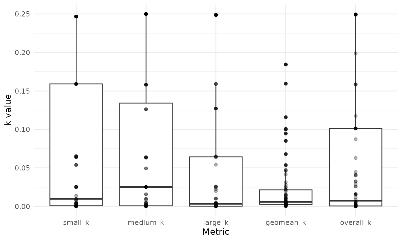
A model-free look at the choice gradient
prop_ss() reports the proportion of smaller-immediate
choices at each of the nine k ranks, pooled across whatever
respondents you pass it. For a single respondent, three items sit at
each rank (one per magnitude), which gives a quick picture of where,
along the discount-rate continuum, that person switches from waiting to
taking the immediate reward:
s1 <- subset(mcq27, subjectid == 1)
prop_ss(s1)
#> # A tibble: 9 × 2
#>    k_rank prop_ss
#>     <dbl>   <dbl>
#> 1 0.00016    1
#> 2 0.0004     1
#> 3 0.001      1
#> 4 0.0025     1
#> 5 0.006      1
#> 6 0.016      1
#> 7 0.041      0.67
#> 8 0.1        0
#> 9 0.25       0
plot(prop_ss(s1))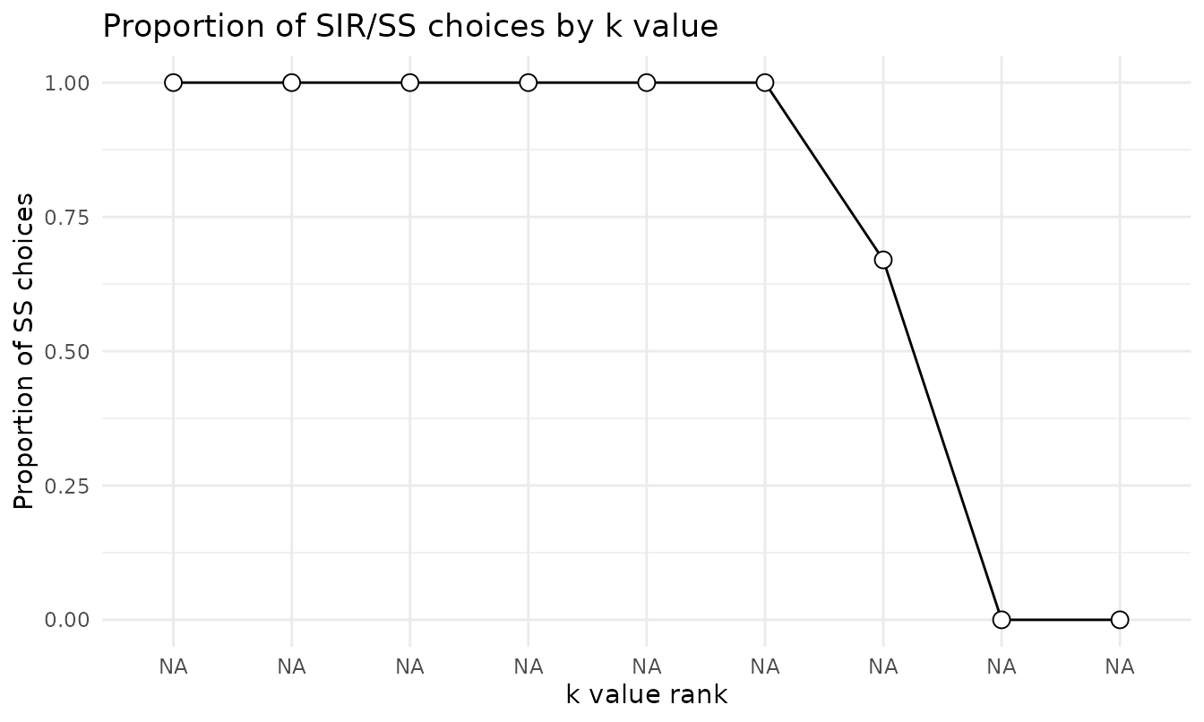
Converting between layouts
Raw MCQ data arrive in different shapes.
wide_to_long_mcq() and long_to_wide_mcq() move
between a wide layout (one column per item) and the long layout
score_mcq27() expects:
wide <- long_to_wide_mcq(mcq27)
dim(wide)
#> [1]  2 28
long <- wide_to_long_mcq(wide)
head(long, 3)
#> # A tibble: 3 × 3
#>   subjectid questionid response
#>       <dbl>      <int>    <dbl>
#> 1         1          1        0
#> 2         1          2        0
#> 3         1          3        0
wide_to_long_mcq_excel() and
long_to_wide_mcq_excel() handle the column layout used by
the published Excel automated scorer, which lets data prepared for that
tool be read in without reformatting.
Handling missing responses
When a respondent leaves items blank, the impute_method
argument controls how the NA responses are handled:
"none" (the default; they stay NA),
"ggm" (geometric grand-mean handling, which drops
NAs when forming geomean_k), or
"inn" (item nearest-neighbor imputation, following Yeh et
al., 2023, which can still leave a value unresolved unless
random = TRUE). Every respondent must still have all 27
items present as rows; impute_method governs only the
NA responses within them, not missing rows.
From choices to trial-level data
Because the MCQ is a choice task, its items can also feed the
structural choice models in beezdiscounting.
mcq27_to_choice() reshapes the responses into the
trial-level frame those models expect:
head(mcq27_to_choice(mcq27))
#> # A tibble: 6 × 5
#>   id    ss_amount ll_amount delay choice
#>   <chr>     <dbl>     <dbl> <dbl>  <dbl>
#> 1 1            54        55   117      0
#> 2 1            55        75    61      0
#> 3 1            19        25    53      0
#> 4 1            31        85     7      1
#> 5 1            14        25    19      1
#> 6 1            47        50   160      0
The result (one row per trial with the smaller and larger amounts,
the delay, and the binary choice) is ready for
fit_dd_choice(). See the choice-modeling and TMB vignettes
for that workflow.
The MCQ has two published versions. Kirby and Marakovic (1996) introduced the original 21-item questionnaire: seven discount-rate ranks, three items per rank except rank 3 (two items, no large-magnitude item) and rank 4 (four items, two of them large), with delayed amounts of $30–$85. Kirby, Petry, and Bickel (1999) extended the design to 27 items across nine evenly populated ranks (three items each, one per magnitude), which is the version scored above. Both versions are scored with the same consistency-maximization logic.
Scoring the 21-item MCQ
The original Monetary Choice Questionnaire (Kirby & Marakovic,
1996) has 21 items over seven discount-rate ranks.
score_mcq() scores it with the same
consistency-maximization algorithm used for the 27-item version:
score_mcq(mcq21, items = 21)
#>   subjectid overall_k  small_k medium_k  large_k geomean_k overall_consistency
#> 1         1  0.006756 0.006878 0.006996 0.004886  0.006172                   1
#> 2         2  0.000700 0.000700 0.000700 0.000700  0.000700                   1
#>   small_consistency medium_consistency large_consistency composite_consistency
#> 1                 1                  1                 1                     1
#> 2                 1                  1                 1                     1
#>   overall_proportion small_proportion medium_proportion large_proportion
#> 1           0.619048         0.571429          0.571429         0.714286
#> 2           1.000000         1.000000          1.000000         1.000000
#>   impute_method
#> 1          none
#> 2          none
Proportions of smaller-sooner choices by rank use the same tooling:
prop_ss(mcq21, items = 21)
#> # A tibble: 7 × 2
#>   k_rank prop_ss
#>    <dbl>   <dbl>
#> 1      1     0.5
#> 2      2     0.5
#> 3      3     0.5
#> 4      4     0
#> 5      5     0
#> 6      6     0
#> 7      7     0
Trial-level modeling works through the same bridge as the 27-item MCQ
(see vignette("choice-discounting")):
head(mcq_to_choice(mcq21, items = 21))
#> # A tibble: 6 × 5
#>   id    ss_amount ll_amount delay choice
#>   <chr>     <dbl>     <dbl> <dbl>  <dbl>
#> 1 1            30        85    14      1
#> 2 1            40        55    25      1
#> 3 1            67        85    35      1
#> 4 1            34        35    43      0
#> 5 1            15        35    10      1
#> 6 1            32        55    20      1
score_mcq27() remains available and is unchanged: it is
now a thin wrapper around score_mcq(), and
score_mcq27(dat) returns exactly
score_mcq(dat, items = 27).
References
- Kaplan, B. A., Amlung, M., Reed, D. D., Jarmolowicz, D. P., McKerchar, T. L., & Lemley, S. M. (2016). Automating scoring of delay discounting for the 21- and 27-item monetary choice questionnaires. The Behavior Analyst, 39, 293–304.
- Kirby, K. N., & Marakovic, N. N. (1996). Delay-discounting probabilistic rewards: Rates decrease as amounts increase. Psychonomic Bulletin & Review, 3(1), 100–104.
- Kirby, K. N., Petry, N. M., & Bickel, W. K. (1999). Heroin addicts have higher discount rates for delayed rewards than non-drug-using controls. Journal of Experimental Psychology: General, 128(1), 78–87.
- Mazur, J. E. (1987). An adjusting procedure for studying delayed reinforcement. In The effect of delay and of intervening events on reinforcement value (pp. 55–73). Lawrence Erlbaum Associates.
- Yeh, Y. H., Tegge, A. N., Freitas-Lemos, R., Myerson, J., Green, L., & Bickel, W. K. (2023). Discounting of delayed rewards: Missing data imputation for the 21- and 27-item monetary choice questionnaires. PLOS ONE, 18(10), e0292258.