Plot a mixed-effects discounting model

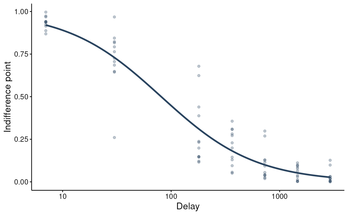
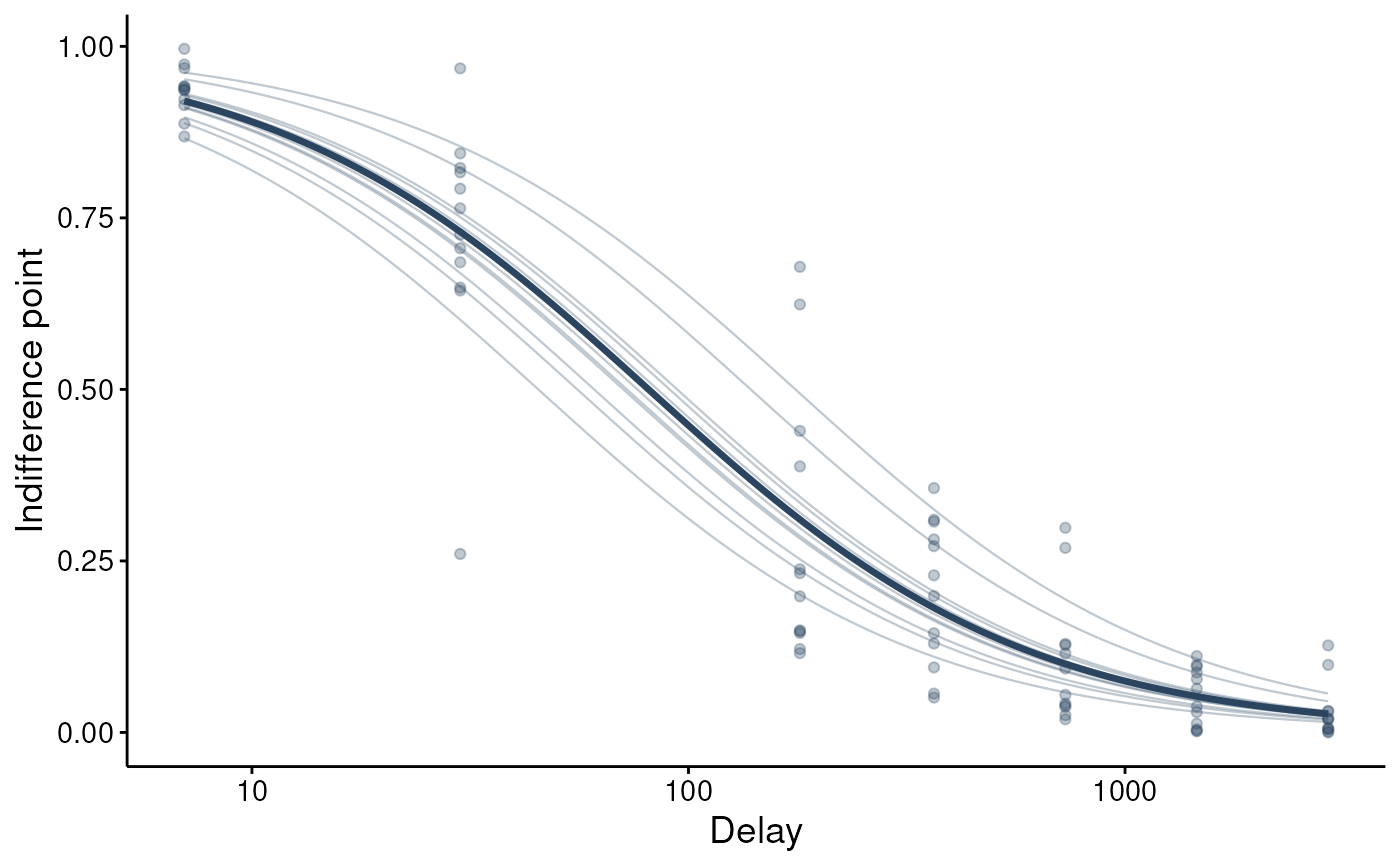
Visualize a fitted fit_dd_tmb() model. type = "population" draws the population (random-effects-at-zero) discount curve over the observed indifference points; type = "individual" adds the per-subject curves (the shrinkage picture). For a fit with factors the population curve is drawn once per factor-level combination; use at to condition on specific levels or covariate values. type = "parameters" shows the distribution of the subject-specific discount rate k (log scale); type = "resid" plots standardized (Pearson) residuals against fitted values.

Usage

# S3 method for class 'beezdiscounting_tmb'
plot(
  x,
  type = c("population", "individual", "parameters", "resid"),
  ids = NULL,
  at = NULL,
  n_points = 200,
  x_trans = c("log10", "linear"),
  show_observed = TRUE,
  ...
)

Arguments

x

A beezdiscounting_tmb object.

type

One of "population", "individual", "parameters", "resid".

ids

Optional subset of subject ids for type = "individual".

at

Optional named list conditioning the population curve on factor levels / covariate values (e.g. list(group = "A")), passed to the same reference-grid machinery as get_dd_comparisons().

n_points

Number of delay points in the curve grid.

x_trans

Delay-axis scale: "log10" (default) or "linear".

show_observed

Overlay the observed indifference points.

...

Unused.

Value

A ggplot2::ggplot object.

Examples

# \donttest{
sim <- simulate_dd_ip(n_subjects = 12, seed = 1)
fit <- fit_dd_tmb(sim, equation = "mazur")
#> Fitting TMB mixed-effects discounting model (mazur, sltb)...
#>   Subjects: 12, Observations: 84
#>   Multi-start: best NLL = -113.59 (start set 3 of 3)
#>   Converged (NLL = -113.59). Done.
plot(fit)

plot(fit, type = "individual")

# }