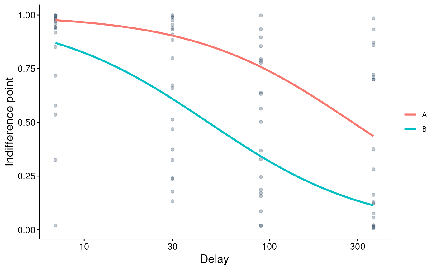
Visualize a fitted fit_dd_linear() model. type = "population" (default)
draws the hyperbola implied by each condition's geometric-mean discount rate
exp(mu) over the observed indifference points (one curve per condition when
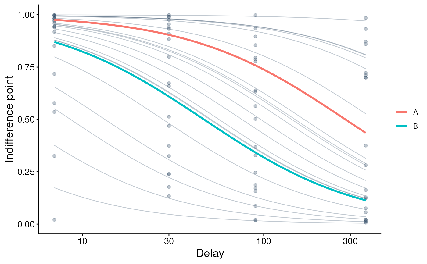
the fit has a factor); type = "individual" adds each subject's own
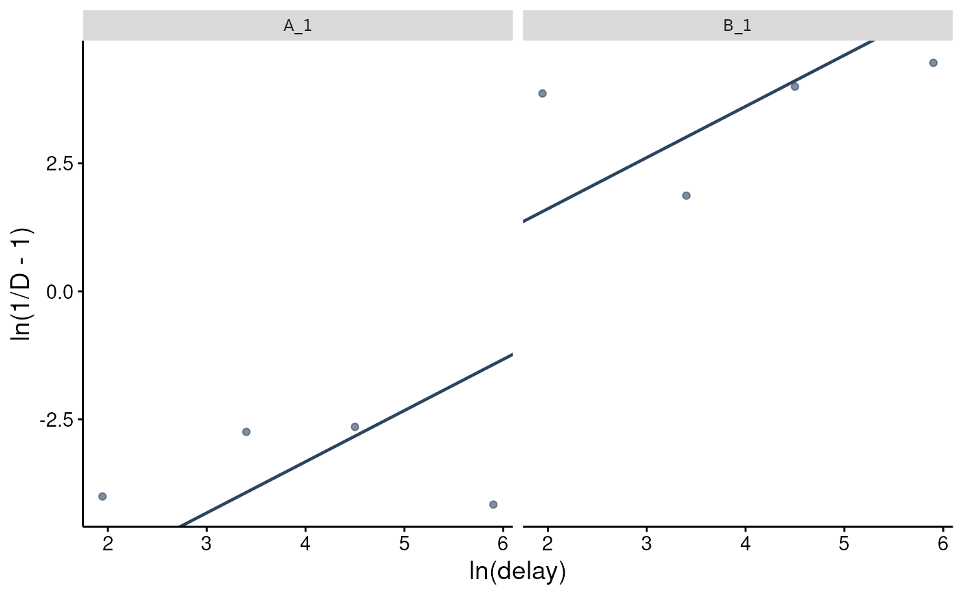
closed-form hyperbola 1 / (1 + k_i x) as thin lines; type = "transformed" shows the linearization itself, ln(1/D - 1) against
ln(delay) per subject with a slope-1 line at that subject's ln k;
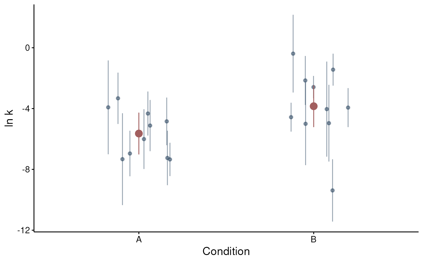
type = "parameters" shows the subject ln k estimates with their
t-intervals (by condition, with the condition mean mu and its interval
from confint() overlaid, when the fit has a factor; otherwise ordered as a
caterpillar), or the same quantities as k on a log10 axis with
k_scale = "log10"; type = "resid" plots the standardized residual on the
transformed scale against ln(delay).
Arguments
- x
A
beezdiscounting_linearobject.- type
One of
"population","individual","transformed","parameters","resid".- ids
Optional subset of subject ids for
type = "individual"andtype = "transformed".- n_points
Number of delay points in the curve grid.
- x_trans
Delay-axis scale:
"log10"(default) or"linear".- show_observed
Overlay the observed indifference points.
- k_scale
For
type = "parameters":"ln"(default) drawsln kon a linear axis;"log10"drawskon a log10 axis as the other tiers do.- ...
Unused.
Value
A ggplot2::ggplot object.
Details
The method shares its core arguments (type, ids, n_points, x_trans,
show_observed) with plot.beezdiscounting_tmb(); it adds k_scale and
omits at (a linearized fit has no covariates or reference grid, so there
is nothing to condition on). x_trans, n_points and show_observed apply to the
"population" and "individual" curves only; ids applies to
"individual" (default: every subject) and "transformed" (default: the
first 12 subjects, with a message when the fit has more).
Unlike the mixed-model tiers there is no shrinkage: every subject's curve is
its own closed-form estimate, and the per-subject pictures do not need the
random-effects component. "population" requires it (the condition means
mu); when the design was unbalanced and re is NULL, "population"
errors, "individual" draws the subject curves only, and "parameters"
omits the condition means with a message.
Two pictures deliberately differ from the mixed-model tiers because this
model is fitted on the linearized scale. "parameters" defaults to ln k
(the scale of coef(), confint() and anova()'s effect size);
k_scale = "log10" gives the sibling tiers' picture, k on a log10 axis.
"resid" plots the transformed-scale residual against ln(delay), the
model's regressor with its slope fixed at 1, so a trend across delay may
indicate delay-dependent lack of fit; the sibling tiers plot
residuals against fitted values instead. k_scale affects only
"parameters".
The "transformed" abscissa is ln(delay) by construction (a log10 axis
would break the slope-1 reference), so x_trans is ignored there.
Indifference points at exactly 0 or 1 are shown at their observed value on
the raw scale, and at their boundary-handled value d_used on the
transformed scale; points dropped under boundary = "drop" do not appear on
the transformed scale. "resid" uses augment()'s .std_resid, the
transformed-scale residual divided by the model's error standard deviation.
Examples
sim <- simulate_dd_linear(
n_subjects = 10, delays = c(7, 30, 90, 365),
mu = c(A = -6, B = -4.5), sigma2 = 2, g = 8, seed = 1
)
fit <- fit_dd_linear(sim, factors = "condition")
plot(fit)
 plot(fit, type = "individual")
 plot(fit, type = "transformed", ids = c("A_1", "B_1"))
 plot(fit, type = "parameters")