Group Comparisons with Extra Sum-of-Squares F-Test

Introduction

When you have multiple groups (e.g., treatment vs. control, different populations), it is often useful to compare whether separate demand curves are preferred over a single curve. The Extra Sum-of-Squares F-test addresses this by fitting a single curve to all data, computing the residual deviations, and comparing those residuals to those obtained from separate group-level curves.

For background on fitting individual demand curves, see vignette("beezdemand"). For mixed-effects approaches to group comparisons, see vignette("mixed-demand").

Note: For formal statistical inference on group differences, mixed-effects models (vignette("mixed-demand")) are the preferred modern approach, offering random effects and estimated marginal means. ExtraF() remains useful for quick, traditional group comparisons.

Setting Up Groups

We will use the built-in apt dataset and manufacture random groupings for demonstration purposes.

## setting the seed initializes the random number generator so results will be
## reproducible
set.seed(1234)

## manufacture random grouping
apt$group <- NA
apt[apt$id %in% sample(unique(apt$id), length(unique(apt$id))/2), "group"] <- "a"
apt$group[is.na(apt$group)] <- "b"

## take a look at what the new groupings look like in long form
knitr::kable(apt[1:20, ])

id	x	y	group
19	0.0	10	a
19	0.5	10	a
19	1.0	10	a
19	1.5	8	a
19	2.0	8	a
19	2.5	8	a
19	3.0	7	a
19	4.0	7	a
19	5.0	7	a
19	6.0	6	a
19	7.0	6	a
19	8.0	5	a
19	9.0	5	a
19	10.0	4	a
19	15.0	3	a
19	20.0	2	a
30	0.0	3	b
30	0.5	3	b
30	1.0	3	b
30	1.5	3	b

Running the Extra Sum-of-Squares F-Test

The ExtraF() function will determine whether a single \alpha or a single Q_0 is better than multiple \alphas or Q_0s. A resulting F statistic will be reported along with a p value.

## in order for this to run, you will have had to run the code immediately
## preceeding (i.e., the code to generate the groups)
ef <- ExtraF(dat = apt, equation = "koff", k = 2, groupcol = "group", verbose = TRUE)

A summary table (broken up here for ease of display) will be created when the option verbose = TRUE. This table can be accessed as the dfres object resulting from ExtraF. In the example above, we can access this summary table using ef$dfres:

Fitted Measures
Group	Q0d	K	R2	Alpha
Shared	NA	NA	NA	NA
a	8.489634	2	0.6206444	0.0040198
b	5.848119	2	0.6206444	0.0040198
Not Shared	NA	NA	NA	NA
a	8.503442	2	0.6448801	0.0040518
b	5.822075	2	0.5242825	0.0039376

Uncertainty and Model Information
Group	N	AbsSS	SdRes
Shared	NA	NA	NA
a	160	387.0945	1.570213
b	160	387.0945	1.570213
Not Shared	NA	NA	NA
a	80	249.2764	1.787695
b	80	137.7440	1.328890

Derived Measures
Group	EV	Omaxd	Pmaxd
Shared	NA	NA	NA
a	0.8795301	22.63159	8.453799
b	0.8795301	22.63159	12.272265
Not Shared	NA	NA	NA
a	0.8725741	22.45260	8.373320
b	0.8978945	23.10414	12.584550

Convergence and Summary Information
Group	Omaxa	Notes
Shared	NA	NA
a	22.63190	converged
b	22.63190	converged
Not Shared	NA	NA
a	22.45291	converged
b	23.10445	converged

Visualizing Group Comparisons

When verbose = TRUE, objects from the result can be used in subsequent graphing. The following code generates a plot of our two groups. We can use the predicted values already generated from the ExtraF function by accessing the newdat object. In the example above, we can access these predicted values using ef$newdat. Note that we keep the linear scaling of y given we used Koffarnus et al. (2015)’s equation fitted to the data.

## be sure that you've loaded the tidyverse package (e.g., library(tidyverse))
ggplot(apt, aes(x = x, y = y, group = group)) +
  ## the predicted lines from the sum of squares f-test can be used in subsequent
  ## plots by calling data = ef$newdat
  geom_line(aes(x = x, y = y, group = group, color = group),
            data = ef$newdat[ef$newdat$x >= .1, ]) +
  stat_summary(fun.data = mean_se, aes(width = .05, color = group),
               geom = "errorbar") +
  stat_summary(fun = mean, aes(fill = group), geom = "point", shape = 21,
               color = "black", stroke = .75, size = 4) +
  scale_x_log10(limits = c(.4, 50), breaks = c(.1, 1, 10, 100)) +
  scale_color_discrete(name = "Group") +
  scale_fill_discrete(name = "Group") +
  labs(x = "Price per Drink", y = "Drinks Purchased") +
  theme(legend.position = c(.85, .75)) +
  ## theme_apa is a beezdemand function used to change the theme in accordance
  ## with American Psychological Association style
  theme_apa()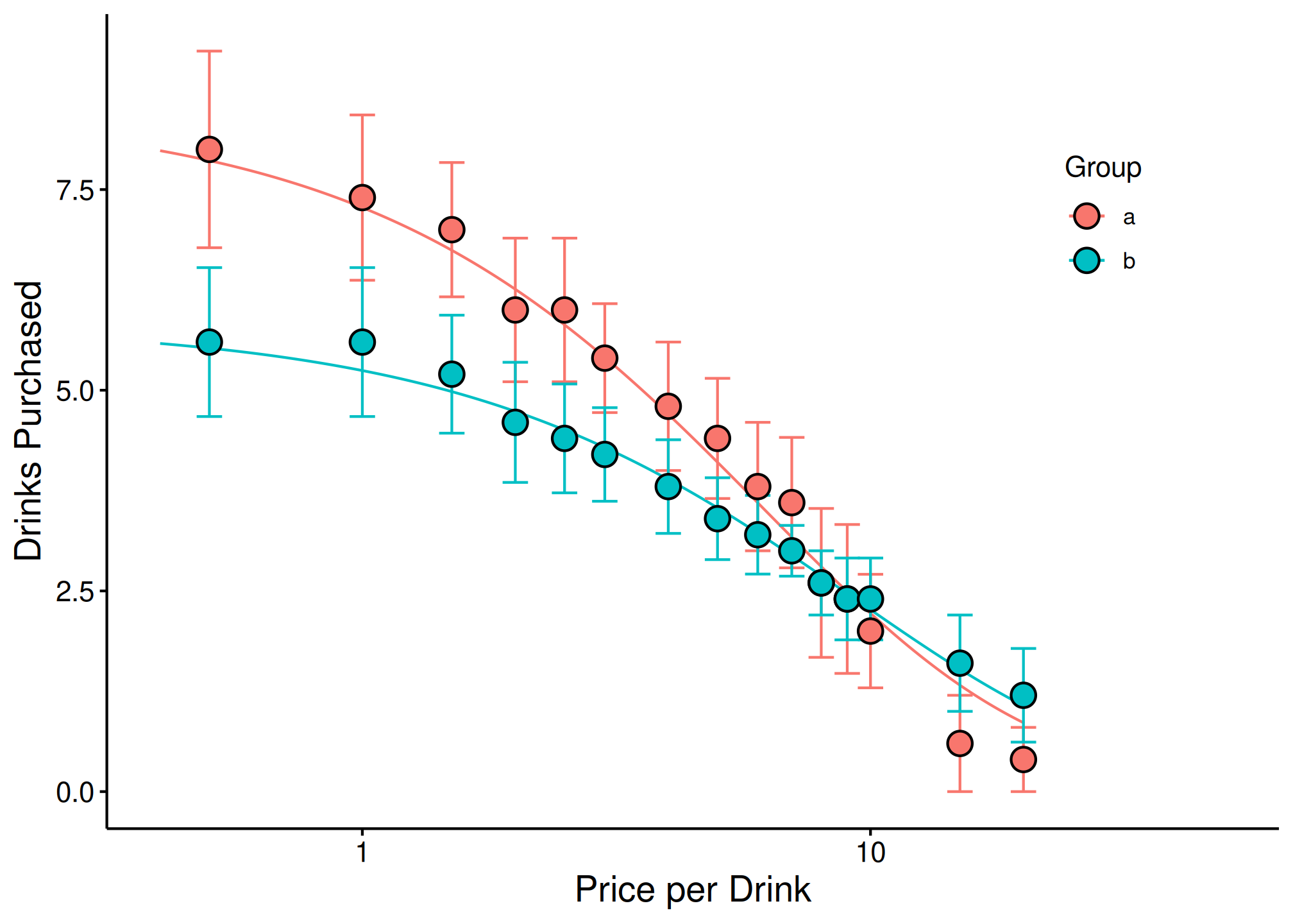

Brent Kaplan

2026-03-03

Introduction

Setting Up Groups

Running the Extra Sum-of-Squares F-Test

Visualizing Group Comparisons

See Also