Choosing the Right Demand Model

Introduction

The beezdemand package provides multiple approaches for fitting behavioral economic demand curves. This guide helps you choose the right modeling approach for your data and research questions.

When to Use Demand Analysis

Demand analysis is appropriate when you want to: - Quantify the value of a reinforcer (e.g., drugs, food, activities) - Compare demand elasticity across conditions or groups - Estimate key parameters like intensity (Q0), elasticity (alpha), and breakpoint - Compute derived metrics like Pmax (price at maximum expenditure) and Omax (maximum expenditure)

Quick Decision Guide

Your Situation	Recommended Approach	Function
Individual curves, quick exploration	Fixed-effects NLS	`fit_demand_fixed()`
Group comparisons, repeated measures	Mixed-effects	`fit_demand_mixed()`
Many zeros, two-part modeling	Hurdle model	`fit_demand_hurdle()`
Cross-commodity substitution	Cross-price models	`fit_cp_*()`

Data Quality First

Before fitting any model, always check your data for systematic responding.

# Check for systematic demand
systematic_check <- check_systematic_demand(apt)
head(systematic_check$results)
#> # A tibble: 6 × 15
#>   id    type   trend_stat trend_threshold trend_direction trend_pass bounce_stat
#>   <chr> <chr>       <dbl>           <dbl> <chr>           <lgl>            <dbl>
#> 1 19    demand      0.211           0.025 down            TRUE                 0
#> 2 30    demand      0.144           0.025 down            TRUE                 0
#> 3 38    demand      0.788           0.025 down            TRUE                 0
#> 4 60    demand      0.909           0.025 down            TRUE                 0
#> 5 68    demand      0.909           0.025 down            TRUE                 0
#> 6 106   demand      0.818           0.025 down            TRUE                 0
#> # ℹ 8 more variables: bounce_threshold <dbl>, bounce_direction <chr>,
#> #   bounce_pass <lgl>, reversals <int>, reversals_pass <lgl>, returns <int>,
#> #   n_positive <int>, systematic <lgl>

# Filter to systematic data only (those that pass all criteria)
systematic_ids <- systematic_check$results |>
  filter(systematic) |>
  dplyr::pull(id)

apt_clean <- apt |>
  filter(as.character(id) %in% systematic_ids)

cat("Systematic participants:", n_distinct(apt_clean$id),
    "of", n_distinct(apt$id), "\n")
#> Systematic participants: 10 of 10

The check_systematic_demand() function applies criteria from Stein et al. (2015) to identify nonsystematic responding patterns including:

Trend (DeltaQ): Consumption should decrease as price increases
Bounce: Limited price-to-price increases in consumption
Reversals: No consumption after sustained zeros

Tier 1: Fixed-Effects NLS

When to Use

Use fit_demand_fixed() when you want:

Individual demand curves for each participant
Quick exploration of your data
Compatibility with traditional analysis approaches
Per-subject parameter estimates without pooling information

Complete Example

# Fit individual demand curves using the Hursh & Silberberg equation
fit_fixed <- fit_demand_fixed(
  data = apt,
  equation = "hs",
  k = 2
)

# Print summary
print(fit_fixed)
#> 
#> Fixed-Effect Demand Model
#> ==========================
#> 
#> Call:
#> fit_demand_fixed(data = apt, equation = "hs", k = 2)
#> 
#> Equation: hs 
#> k: fixed (2) 
#> Subjects: 10 ( 10 converged, 0 failed)
#> 
#> Use summary() for parameter summaries, tidy() for tidy output.

# Get tidy coefficient table
tidy(fit_fixed) |> head()
#> # A tibble: 6 × 10
#>   id    term  estimate std.error statistic p.value component estimate_scale
#>   <chr> <chr>    <dbl>     <dbl>     <dbl>   <dbl> <chr>     <chr>         
#> 1 19    Q0       10.2      0.269        NA      NA fixed     natural       
#> 2 30    Q0        2.81     0.226        NA      NA fixed     natural       
#> 3 38    Q0        4.50     0.215        NA      NA fixed     natural       
#> 4 60    Q0        9.92     0.459        NA      NA fixed     natural       
#> 5 68    Q0       10.4      0.329        NA      NA fixed     natural       
#> 6 106   Q0        5.68     0.300        NA      NA fixed     natural       
#> # ℹ 2 more variables: term_display <chr>, estimate_internal <dbl>

# Get model-level statistics
glance(fit_fixed)
#> # A tibble: 1 × 12
#>   model_class      backend equation k_spec     nobs n_subjects n_success n_fail
#>   <chr>            <chr>   <chr>    <chr>     <int>      <int>     <int>  <int>
#> 1 beezdemand_fixed legacy  hs       fixed (2)   146         10        10      0
#> # ℹ 4 more variables: converged <lgl>, logLik <dbl>, AIC <dbl>, BIC <dbl>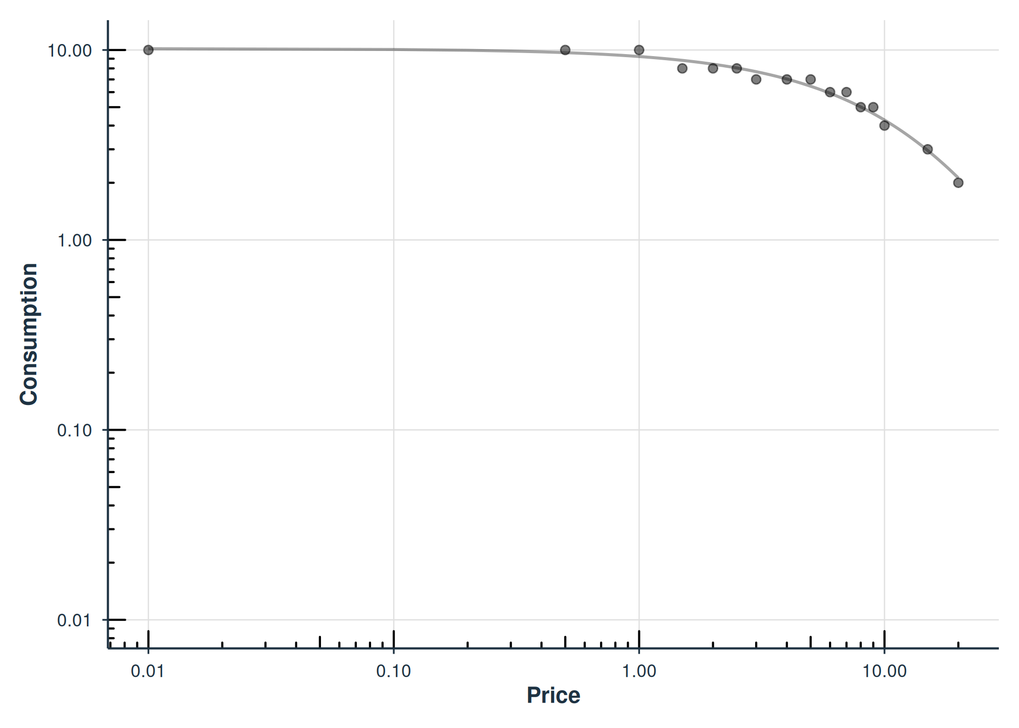

# Plot individual curves
plot(fit_fixed, type = "individual", ids = c("19", "51"))

Individual demand curves for two example participants.

# Basic diagnostics
check_demand_model(fit_fixed)
#> 
#> Model Diagnostics
#> ================================================== 
#> Model class: beezdemand_fixed 
#> 
#> Convergence:
#>   Status: Converged
#> 
#> Residuals:
#>   Mean: 0.0284
#>   SD: 0.5306
#>   Range: [-1.458, 2.228]
#>   Outliers: 3 observations
#> 
#> --------------------------------------------------
#> Issues Detected (1):
#>   1. Detected 3 potential outliers across subjects

Tier 2: Mixed-Effects Models

When to Use

Use fit_demand_mixed() when you want:

Group comparisons with statistical inference
Random effects to account for individual variability
Post-hoc comparisons between conditions
Estimated marginal means for factor levels

The LL4 Transformation

For the mixed-effects approach with the zben equation form, transform your consumption data using the LL4 (log-log with 4-parameter adjustment):

# Transform consumption using LL4
apt_ll4 <- apt |>
  dplyr::mutate(y_ll4 = ll4(y))

# View the transformation
apt_ll4 |>
  dplyr::filter(id == 19) |>
  dplyr::select(id, x, y, y_ll4)

Complete Example

# Fit mixed-effects model
fit_mixed <- fit_demand_mixed(
  data = apt_ll4,
  y_var = "y_ll4",
  x_var = "x",
  id_var = "id",
  equation_form = "zben"
)

# Print summary
print(fit_mixed)
summary(fit_mixed)

# Basic diagnostics
check_demand_model(fit_mixed)
plot_residuals(fit_mixed)$fitted

Post-Hoc Analysis with emmeans

For experimental designs with factors, you can use emmeans for post-hoc comparisons:

# For a model with factors (example with ko dataset):
data(ko)

# Prepare data with LL4 transformation
# (Note: the ko dataset already includes a y_ll4 column, but we
# recreate it here to demonstrate the transformation workflow)
ko_ll4 <- ko |>
  dplyr::mutate(y_ll4 = ll4(y))

fit <- fit_demand_mixed(
  data = ko_ll4,
  y_var = "y_ll4",
  x_var = "x",
  id_var = "monkey",
  factors = c("drug", "dose"),
  equation_form = "zben"
)

# Get estimated marginal means for Q0 and alpha across drug levels
emms <- get_demand_param_emms(fit, factors_in_emm = "drug", include_ev = TRUE)

# Pairwise comparisons of drug conditions
comps <- get_demand_comparisons(fit, compare_specs = ~drug, contrast_type = "pairwise")

Tier 3: Hurdle Models

When to Use

Use fit_demand_hurdle() when you have:

Substantial zero consumption values (>10-15% zeros)
Need for two-part modeling (zeros vs. positive consumption)
Interest in both participation and consumption intensity
TMB backend for fast, stable estimation

Understanding the Two-Part Structure

The hurdle model separates:

Part I: Probability of zero consumption (logistic regression)
Part II: Log-consumption given positive response (nonlinear mixed effects)

Complete Example

# Fit hurdle model with 3 random effects
fit_hurdle <- fit_demand_hurdle(
  data = apt,
  y_var = "y",
  x_var = "x",
  id_var = "id",
  random_effects = c("zeros", "q0", "alpha")
)

# Summary
summary(fit_hurdle)

# Population demand curve
plot(fit_hurdle, type = "demand")

# Probability of zero consumption
plot(fit_hurdle, type = "probability")

# Basic diagnostics
check_demand_model(fit_hurdle)
plot_residuals(fit_hurdle)$fitted
plot_qq(fit_hurdle)

Comparing Hurdle Models

Compare nested models using likelihood ratio tests:

# Fit full model (3 random effects)
fit_hurdle3 <- fit_demand_hurdle(
  data = apt,
  y_var = "y",
  x_var = "x",
  id_var = "id",
  random_effects = c("zeros", "q0", "alpha")
)

# Fit simplified model (2 random effects)
fit_hurdle2 <- fit_demand_hurdle(
  data = apt,
  y_var = "y",
  x_var = "x",
  id_var = "id",
  random_effects = c("zeros", "q0")  # No alpha random effect
)

# Compare models
compare_hurdle_models(fit_hurdle3, fit_hurdle2)

# Unified model comparison (AIC/BIC + LRT when appropriate)
compare_models(fit_hurdle3, fit_hurdle2)

Choosing an Equation

The equation argument determines the functional form of the demand curve. Each equation has trade-offs in terms of flexibility, zero handling, and comparability across studies.

Equation	Function	Handles Zeros	k Required	Best For
`"hs"`	Hursh & Silberberg (2008)	No	Yes	Traditional analyses, compatibility with older literature
`"koff"`	Koffarnus et al. (2015)	No	Yes	Modified exponential, widely used in applied research
`"simplified"`	Rzeszutek et al. (2025)	Yes	No	Modern analyses; avoids k-dependency and zero issues

Recommendations:

For new analyses, consider using "simplified" (also called SND) as it handles zeros natively and does not require specifying k, making results more comparable across studies.
For replication or comparability with existing literature, use "hs" or "koff" with the same k specification as the original study.
When using "hs" or "koff", zeros in consumption data are incompatible with the log transformation and will be dropped with a warning.

Choosing Parameters

The k Parameter

The scaling constant k controls the asymptotic range of the demand curve:

k = 2: Good default for most purchase task data
k = "ind": Calculate k individually for each participant
k = "fit": Estimate k as a free parameter
k = "share": Fit a single k shared across all participants

# Different k specifications
fit_k2 <- fit_demand_fixed(apt, k = 2)          # Fixed at 2
fit_kind <- fit_demand_fixed(apt, k = "ind")    # Individual
fit_kfit <- fit_demand_fixed(apt, k = "fit")    # Free parameter
fit_kshare <- fit_demand_fixed(apt, k = "share") # Shared across participants

Interpreting Key Parameters

Parameter	Interpretation	Typical Range
Q0 (Intensity)	Consumption at zero price	Dataset-dependent
alpha (Elasticity)	Rate of consumption decline	0.0001 - 0.1
Pmax	Price at maximum expenditure	Dataset-dependent
Omax	Maximum expenditure	Dataset-dependent
Breakpoint	First price with zero consumption	Dataset-dependent

Troubleshooting FAQ

Model Convergence Issues

Problem: Model fails to converge or produces unreasonable estimates.

Solutions:

Check data quality with check_systematic_demand()
Try different starting values
Use a simpler model (fewer random effects)
Ensure sufficient data per participant

Zero Handling

Problem: Many zeros in consumption data.

Solutions:

Use fit_demand_hurdle() which explicitly models zeros
For fixed-effects: zeros are automatically excluded for log-transformed equations
Consider data quality: excessive zeros may indicate nonsystematic responding

Parameter Comparison Across Models

Problem: Comparing alpha values between different model types.

Solution: Be aware of parameterization differences:

Hurdle models estimate on natural-log scale internally
Use tidy(fit, report_space = "log10") for comparable output
The transformation is: log10(alpha) = log(alpha) / log(10)

Summary

Approach	Best For	Key Features	Handles Zeros
`fit_demand_fixed()`	Individual curves, quick analysis	Simple, per-subject estimates	Excludes
`fit_demand_mixed()`	Group comparisons, repeated measures	Random effects, emmeans integration	LL4 transform
`fit_demand_hurdle()`	Data with many zeros	Two-part model, TMB backend	Explicitly models

Next Steps

Getting Started: See vignette("beezdemand") for basic usage
Fixed-Effect Models: See vignette("fixed-demand") for individual demand curve fitting
Group Comparisons: See vignette("group-comparisons") for extra sum-of-squares F-test
Mixed Models: See vignette("mixed-demand") for mixed-effects examples
Advanced Mixed Models: See vignette("mixed-demand-advanced") for factors, EMMs, covariates
Hurdle Models: See vignette("hurdle-demand-models") for hurdle model details
Cross-Price: See vignette("cross-price-models") for substitution analyses
Migration Guide: See vignette("migration-guide") for migrating from FitCurves()

References

Hursh, S. R., & Silberberg, A. (2008). Economic demand and essential value. Psychological Review, 115(1), 186-198.
Koffarnus, M. N., Franck, C. T., Stein, J. S., & Bickel, W. K. (2015). A modified exponential behavioral economic demand model to better describe consumption data. Experimental and Clinical Psychopharmacology, 23(6), 504-512.
Stein, J. S., Koffarnus, M. N., Snider, S. E., Quisenberry, A. J., & Bickel, W. K. (2015). Identification and management of nonsystematic purchase task data: Toward best practice. Experimental and Clinical Psychopharmacology, 23(5), 377-386.
Kaplan, B. A., Franck, C. T., McKee, K., Gilroy, S. P., & Koffarnus, M. N. (2021). Applying mixed-effects modeling to behavioral economic demand: An introduction. Perspectives on Behavior Science, 44(2), 333-358.
Rzeszutek, M. J., Regnier, S. D., Franck, C. T., & Koffarnus, M. N. (2025). Overviewing the exponential model of demand and introducing a simplification that solves issues of span, scale, and zeros. Experimental and Clinical Psychopharmacology.

Brent Kaplan

2026-03-03

Introduction

When to Use Demand Analysis

Quick Decision Guide

Data Quality First

Tier 1: Fixed-Effects NLS

When to Use

Complete Example

Tier 2: Mixed-Effects Models

When to Use

The LL4 Transformation

Complete Example

Post-Hoc Analysis with emmeans

Tier 3: Hurdle Models

When to Use

Understanding the Two-Part Structure

Complete Example

Comparing Hurdle Models

Choosing an Equation

Choosing Parameters

The k Parameter

Interpreting Key Parameters

Troubleshooting FAQ

Model Convergence Issues

Zero Handling

Parameter Comparison Across Models

Summary

Next Steps

References