Fixed-Effect Demand Modeling with `beezdemand`
Brent Kaplan
2026-06-24
Source:vignettes/fixed-demand.Rmd
fixed-demand.RmdIntroduction
This vignette demonstrates how to fit individual (fixed-effect)
demand curves using fit_demand_fixed(). This function fits
separate nonlinear least squares (NLS) models for each subject,
producing per-subject estimates of demand parameters like Q_{0} (intensity) and \alpha (elasticity).
When to use fixed-effect models: Fixed-effect models
are appropriate when you want independent curve fits for each
participant. They make no assumptions about the distribution of
parameters across subjects and are the simplest approach to demand curve
analysis. For hierarchical models that share information across
subjects, see vignette("mixed-demand"). For guidance on
choosing between approaches, see
vignette("model-selection").
Data format: All modeling functions expect
long-format data with columns id (subject identifier),
x (price), and y (consumption). See
vignette("beezdemand") for details on data preparation and
conversion from wide format.
Fitting with Different Equations
fit_demand_fixed() supports several equation forms. We
demonstrate the three most common below using the apt
(Alcohol Purchase Task) dataset.
Hursh & Silberberg (“hs”)
The exponential model of demand (Hursh & Silberberg, 2008):
\log_{10}(Q) = \log_{10}(Q_0) + k \cdot (e^{-\alpha \cdot Q_0 \cdot x} - 1)
fit_hs <- fit_demand_fixed(apt, equation = "hs", k = 2)
fit_hs
#>
#> Fixed-Effect Demand Model
#> ==========================
#>
#> Call:
#> fit_demand_fixed(data = apt, equation = "hs", k = 2)
#>
#> Equation: hs
#> k: fixed (2)
#> Subjects: 10 ( 10 converged, 0 failed)
#>
#> Use summary() for parameter summaries, tidy() for tidy output.
Koffarnus (“koff”)
The exponentiated model (Koffarnus et al., 2015):
Q = Q_0 \cdot 10^{k \cdot (e^{-\alpha \cdot Q_0 \cdot x} - 1)}
fit_koff <- fit_demand_fixed(apt, equation = "koff", k = 2)
fit_koff
#>
#> Fixed-Effect Demand Model
#> ==========================
#>
#> Call:
#> fit_demand_fixed(data = apt, equation = "koff", k = 2)
#>
#> Equation: koff
#> k: fixed (2)
#> Subjects: 10 ( 10 converged, 0 failed)
#>
#> Use summary() for parameter summaries, tidy() for tidy output.
Simplified (“simplified”)
The simplified exponential model (Rzeszutek et al., 2025) does not require a scaling constant k:
Q = Q_0 \cdot e^{-\alpha \cdot Q_0 \cdot x}
fit_simplified <- fit_demand_fixed(apt, equation = "simplified")
fit_simplified
#>
#> Fixed-Effect Demand Model
#> ==========================
#>
#> Call:
#> fit_demand_fixed(data = apt, equation = "simplified")
#>
#> Equation: simplified
#> k: none (simplified equation)
#> Subjects: 10 ( 10 converged, 0 failed)
#>
#> Use summary() for parameter summaries, tidy() for tidy output.
The k Parameter
The scaling constant k controls the
range of the demand function. For the "hs" and
"koff" equations, k can be specified in
several ways:
k value |
Behavior |
|---|---|
Numeric (e.g., 2) |
Fixed constant for all subjects (default) |
"ind" |
Individual k per subject, computed from each subject’s data range |
"share" |
Single shared k estimated across all subjects via global regression |
"fit" |
k is a free parameter estimated jointly with Q_0 and \alpha |
## Fixed k (default)
fit_demand_fixed(apt, equation = "hs", k = 2)

## Individual k per subject
fit_demand_fixed(apt, equation = "hs", k = "ind")

## Shared k across subjects
fit_demand_fixed(apt, equation = "hs", k = "share")

## Fitted k as free parameter
fit_demand_fixed(apt, equation = "hs", k = "fit")
The param_space argument controls whether optimization
is performed on the natural scale ("natural", the default)
or log10 scale ("log10"). The log10 scale can improve
convergence for some datasets:
fit_demand_fixed(apt, equation = "hs", k = 2, param_space = "log10")Inspecting Fits
All beezdemand_fixed objects support the standard
tidy(), glance(), augment(), and
confint() methods for programmatic access to results.
tidy(): Per-Subject Parameter Estimates
tidy(fit_hs)
#> # A tibble: 40 × 10
#>    id    term  estimate std.error statistic p.value component estimate_scale
#>    <chr> <chr>    <dbl>     <dbl>     <dbl>   <dbl> <chr>     <chr>
#>  1 19    Q0       10.2      0.269        NA      NA fixed     natural
#>  2 30    Q0        2.81     0.226        NA      NA fixed     natural
#>  3 38    Q0        4.50     0.215        NA      NA fixed     natural
#>  4 60    Q0        9.92     0.459        NA      NA fixed     natural
#>  5 68    Q0       10.4      0.329        NA      NA fixed     natural
#>  6 106   Q0        5.68     0.300        NA      NA fixed     natural
#>  7 113   Q0        6.20     0.174        NA      NA fixed     natural
#>  8 142   Q0        6.17     0.641        NA      NA fixed     natural
#>  9 156   Q0        8.35     0.411        NA      NA fixed     natural
#> 10 188   Q0        6.30     0.564        NA      NA fixed     natural
#> # ℹ 30 more rows
#> # ℹ 2 more variables: term_display <chr>, estimate_internal <dbl>
glance(): Model-Level Summary
glance(fit_hs)
#> # A tibble: 1 × 12
#>   model_class      backend equation k_spec     nobs n_subjects n_success n_fail
#>   <chr>            <chr>   <chr>    <chr>     <int>      <int>     <int>  <int>
#> 1 beezdemand_fixed legacy  hs       fixed (2)   146         10        10      0
#> # ℹ 4 more variables: converged <lgl>, logLik <dbl>, AIC <dbl>, BIC <dbl>
augment(): Fitted Values and Residuals
augment(fit_hs)
#> # A tibble: 146 × 6
#>    id        x     y     k .fitted  .resid
#>    <chr> <dbl> <dbl> <dbl>   <dbl>   <dbl>
#>  1 19      0      10     2   10.2  -0.159
#>  2 19      0.5    10     2    9.69  0.314
#>  3 19      1      10     2    9.24  0.760
#>  4 19      1.5     8     2    8.82 -0.819
#>  5 19      2       8     2    8.42 -0.421
#>  6 19      2.5     8     2    8.04 -0.0444
#>  7 19      3       7     2    7.69 -0.689
#>  8 19      4       7     2    7.03 -0.0334
#>  9 19      5       7     2    6.45  0.554
#> 10 19      6       6     2    5.92  0.0820
#> # ℹ 136 more rows
confint(): Confidence Intervals
confint(fit_hs)
#> # A tibble: 40 × 6
#>    id    term  estimate conf.low conf.high level
#>    <chr> <chr>    <dbl>    <dbl>     <dbl> <dbl>
#>  1 19    Q0       10.2      9.63     10.7   0.95
#>  2 30    Q0        2.81     2.36      3.25  0.95
#>  3 38    Q0        4.50     4.08      4.92  0.95
#>  4 60    Q0        9.92     9.02     10.8   0.95
#>  5 68    Q0       10.4      9.75     11.0   0.95
#>  6 106   Q0        5.68     5.10      6.27  0.95
#>  7 113   Q0        6.20     5.85      6.54  0.95
#>  8 142   Q0        6.17     4.92      7.43  0.95
#>  9 156   Q0        8.35     7.54      9.15  0.95
#> 10 188   Q0        6.30     5.20      7.41  0.95
#> # ℹ 30 more rows
summary(): Formatted Summary
The summary() method provides a formatted overview
including parameter distributions across subjects:
summary(fit_hs)
#>
#> Fixed-Effect Demand Model Summary
#> ==================================================
#>
#> Equation: hs
#> k: fixed (2)
#>
#> Fit Summary:
#>   Total subjects: 10
#>   Converged: 10
#>   Failed: 0
#>   Total observations: 146
#>
#> Parameter Summary (across subjects):
#>   Q0:
#>     Median: 6.2498
#>     Range: [ 2.8074 , 10.3904 ]
#>   alpha:
#>     Median: 0.004251
#>     Range: [ 0.001987 , 0.00785 ]
#>
#> Per-subject coefficients:
#> -------------------------
#> # A tibble: 40 × 10
#>    id    term      estimate std.error statistic p.value component estimate_scale
#>    <chr> <chr>        <dbl>     <dbl>     <dbl>   <dbl> <chr>     <chr>
#>  1 106   Q0         5.68     0.300           NA      NA fixed     natural
#>  2 106   alpha      0.00628  0.000432        NA      NA fixed     natural
#>  3 106   alpha_st…  0.0257   0.00176         NA      NA fixed     natural
#>  4 106   k          2       NA               NA      NA fixed     natural
#>  5 113   Q0         6.20     0.174           NA      NA fixed     natural
#>  6 113   alpha      0.00199  0.000109        NA      NA fixed     natural
#>  7 113   alpha_st…  0.00812  0.000447        NA      NA fixed     natural
#>  8 113   k          2       NA               NA      NA fixed     natural
#>  9 142   Q0         6.17     0.641           NA      NA fixed     natural
#> 10 142   alpha      0.00237  0.000400        NA      NA fixed     natural
#> # ℹ 30 more rows
#> # ℹ 2 more variables: term_display <chr>, estimate_internal <dbl>
Normalized Alpha (\alpha^*)
When k varies across participants or
studies (e.g., k = "ind" or k = "fit"), raw
\alpha values are not directly
comparable. The alpha_star column in tidy()
output provides a normalized version (Strategy B; Rzeszutek et al.,
2025) that adjusts for the scaling constant:
\alpha^* = \frac{-\alpha}{\ln\!\left(1 - \frac{1}{k \cdot \ln(b)}\right)}
where b is the logarithmic base (10
for HS/Koff equations). Standard errors are computed via the delta
method. alpha_star requires k
\cdot \ln(b) > 1; otherwise NA is returned.
tidy(fit_hs) |>
  filter(term == "alpha_star") |>
  select(id, term, estimate, std.error)
#> # A tibble: 10 × 4
#>    id    term       estimate std.error
#>    <chr> <chr>         <dbl>     <dbl>
#>  1 19    alpha_star  0.00836  0.000249
#>  2 30    alpha_star  0.0240   0.00276
#>  3 38    alpha_star  0.0172   0.00146
#>  4 60    alpha_star  0.0176   0.000592
#>  5 68    alpha_star  0.0113   0.000394
#>  6 106   alpha_star  0.0257   0.00176
#>  7 113   alpha_star  0.00812  0.000447
#>  8 142   alpha_star  0.00969  0.00163
#>  9 156   alpha_star  0.0193   0.000668
#> 10 188   alpha_star  0.0321   0.00184
Plotting
Basic Demand Curves
The plot() method displays fitted demand curves with
observed data points. The x-axis defaults to a log10 scale:
plot(fit_hs)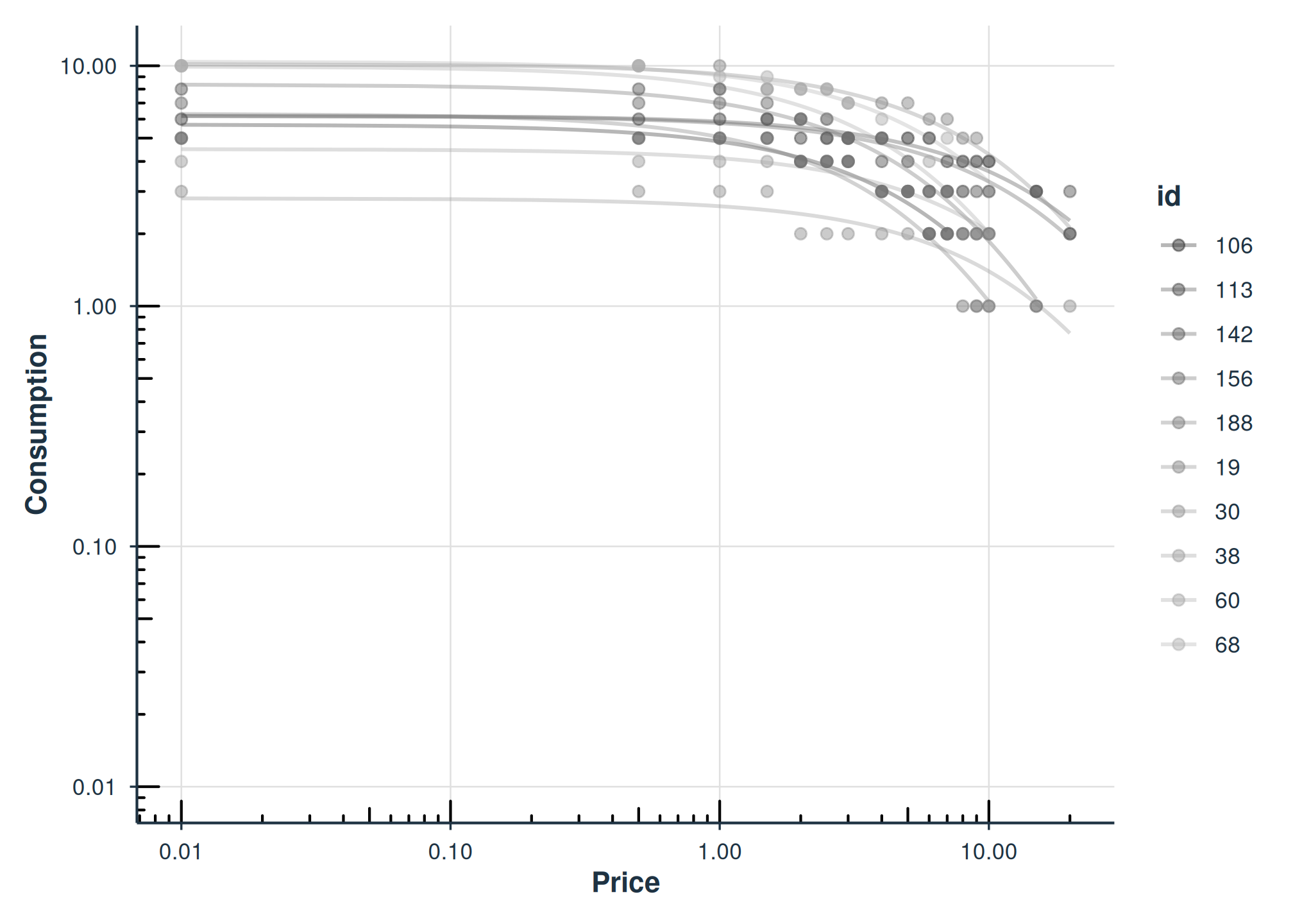
Faceted by Subject
Use facet = TRUE to show each subject in a separate
panel:
plot(fit_hs, facet = TRUE)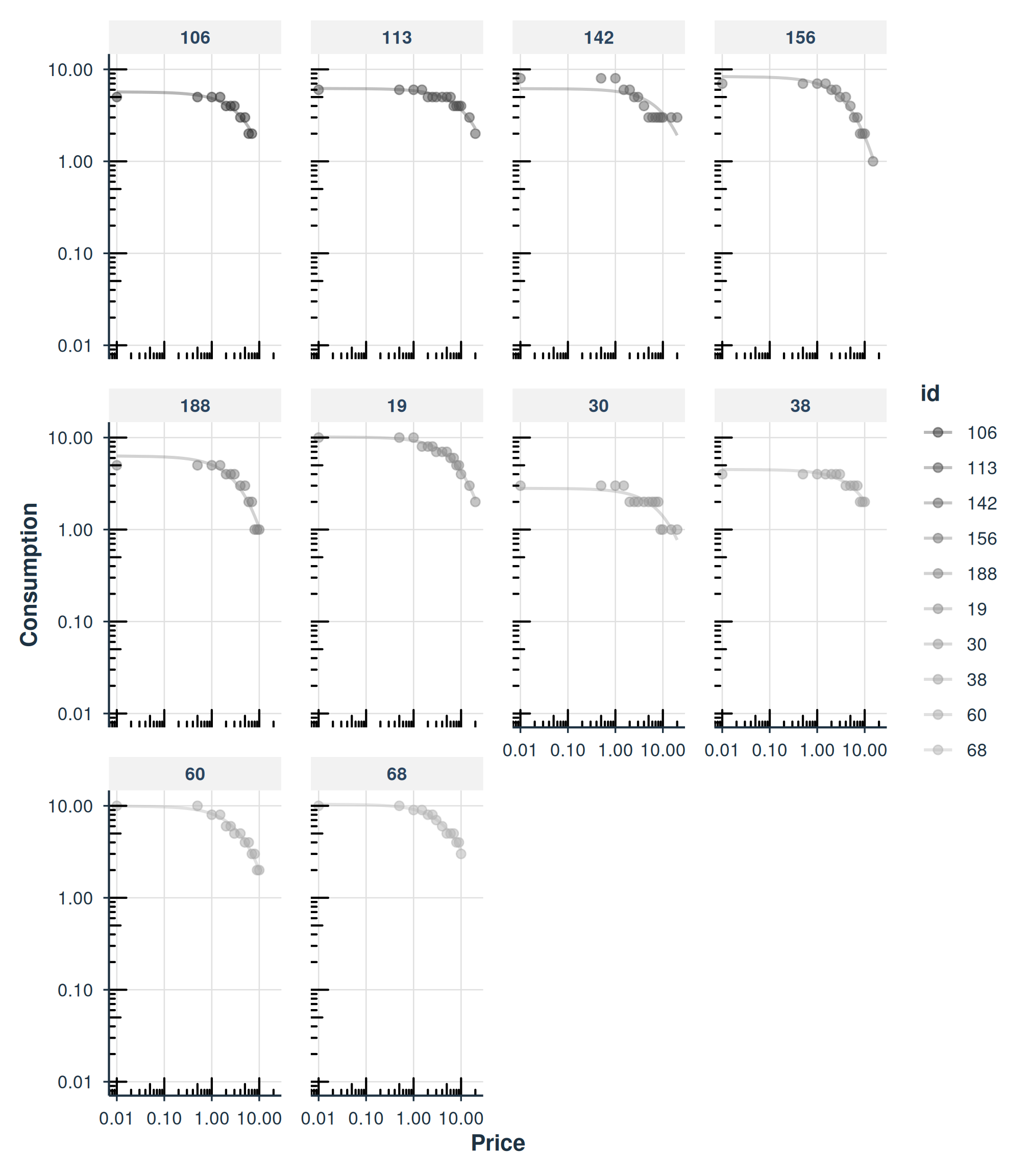
Axis Transformations
Control the x- and y-axis transformations with x_trans
and y_trans:
plot(fit_hs, x_trans = "pseudo_log", y_trans = "pseudo_log")![]()
Diagnostics
Model Checks
check_demand_model() summarizes convergence, residual
properties, and potential issues:
check_demand_model(fit_hs)
#>
#> Model Diagnostics
#> ==================================================
#> Model class: beezdemand_fixed
#>
#> Convergence:
#>   Status: Converged
#>
#> Residuals:
#>   Mean: 0.0284
#>   SD: 0.5306
#>   Range: [-1.458, 2.228]
#>   Outliers: 3 observations
#>
#> --------------------------------------------------
#> Issues Detected (1):
#>   1. Detected 3 potential outliers across subjects
Residual Plots
plot_residuals() produces diagnostic plots. Use
$fitted for a residuals-vs-fitted plot:
plot_residuals(fit_hs)$fitted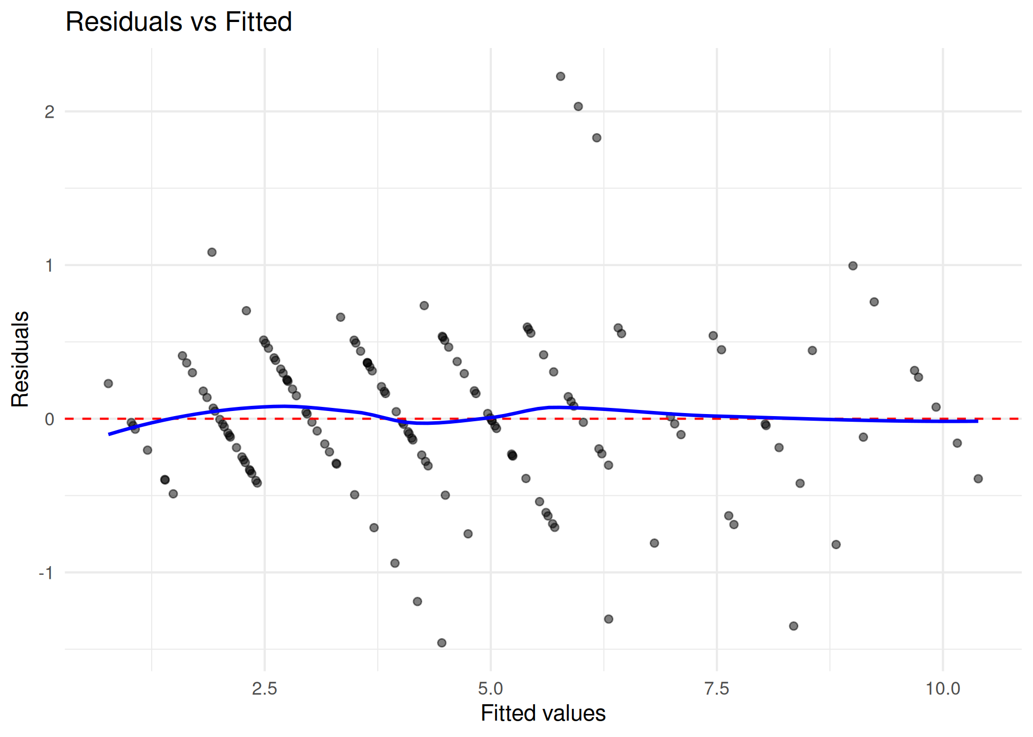
Predictions
Default Predictions
predict() with no arguments returns fitted values at the
observed prices:
predict(fit_hs)
#> # A tibble: 160 × 3
#>        x id    .fitted
#>    <dbl> <chr>   <dbl>
#>  1     0 19      10.2
#>  2     0 30       2.81
#>  3     0 38       4.50
#>  4     0 60       9.92
#>  5     0 68      10.4
#>  6     0 106      5.68
#>  7     0 113      6.20
#>  8     0 142      6.17
#>  9     0 156      8.35
#> 10     0 188      6.30
#> # ℹ 150 more rows
Custom Price Grid
Supply newdata to predict at specific prices:
new_prices <- data.frame(x = c(0, 0.5, 1, 2, 5, 10, 20))
predict(fit_hs, newdata = new_prices)
#> # A tibble: 70 × 3
#>        x id    .fitted
#>    <dbl> <chr>   <dbl>
#>  1     0 19      10.2
#>  2     0 30       2.81
#>  3     0 38       4.50
#>  4     0 60       9.92
#>  5     0 68      10.4
#>  6     0 106      5.68
#>  7     0 113      6.20
#>  8     0 142      6.17
#>  9     0 156      8.35
#> 10     0 188      6.30
#> # ℹ 60 more rows
Aggregated Models
Instead of fitting each subject individually, you can fit a single curve to aggregated data.
Mean Aggregation
agg = "Mean" computes the mean consumption at each price
across subjects, then fits a single curve to those means:
fit_mean <- fit_demand_fixed(apt, equation = "hs", k = 2, agg = "Mean")
fit_mean
#>
#> Fixed-Effect Demand Model
#> ==========================
#>
#> Call:
#> fit_demand_fixed(data = apt, equation = "hs", k = 2, agg = "Mean")
#>
#> Equation: hs
#> k: fixed (2)
#> Aggregation: Mean
#> Subjects: 1 ( 1 converged, 0 failed)
#>
#> Use summary() for parameter summaries, tidy() for tidy output.
plot(fit_mean)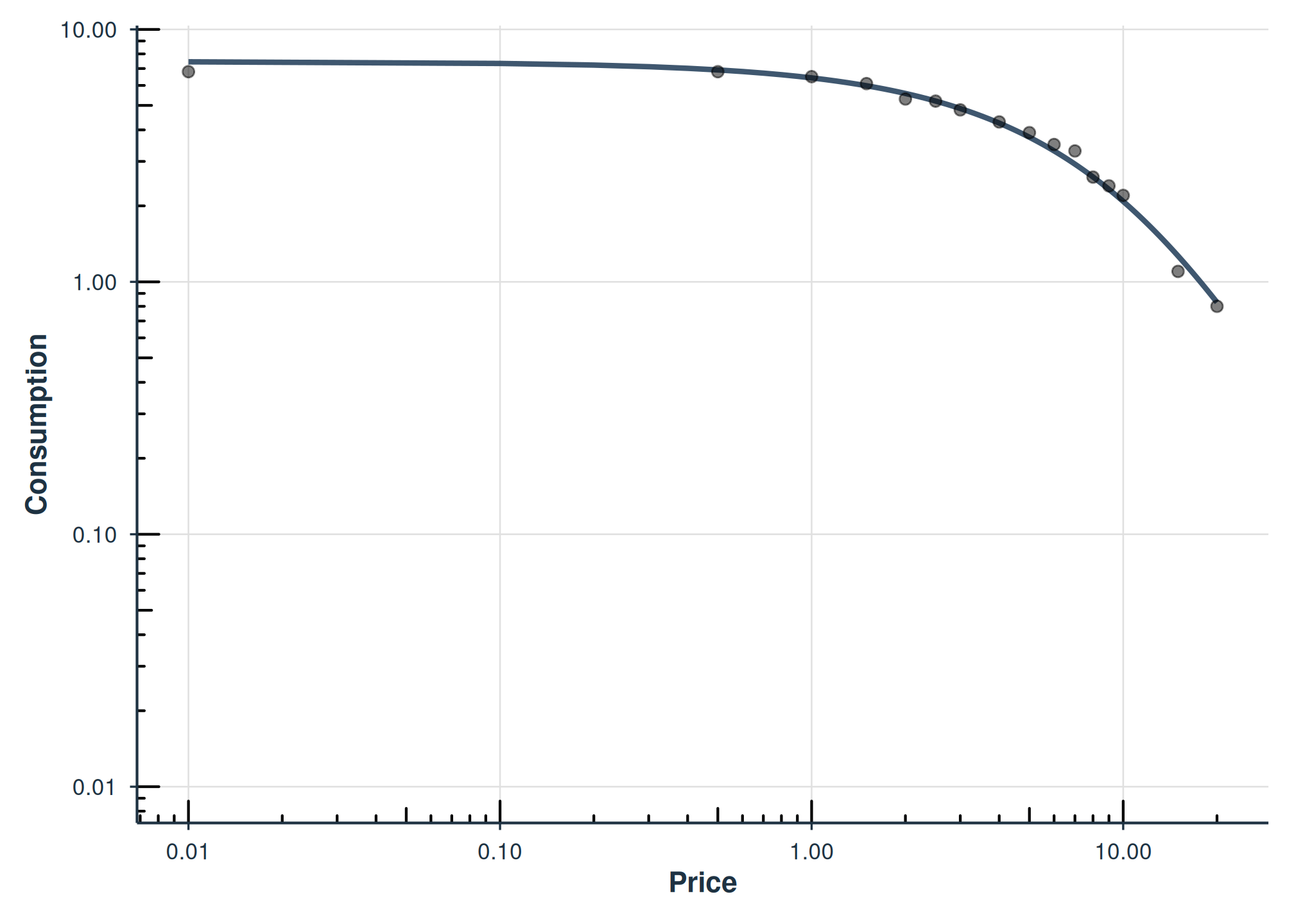
Pooled Aggregation
agg = "Pooled" fits a single curve to all data points
pooled together, retaining error around each observation but ignoring
within-subject clustering:
fit_pooled <- fit_demand_fixed(apt, equation = "hs", k = 2, agg = "Pooled")
fit_pooled
#>
#> Fixed-Effect Demand Model
#> ==========================
#>
#> Call:
#> fit_demand_fixed(data = apt, equation = "hs", k = 2, agg = "Pooled")
#>
#> Equation: hs
#> k: fixed (2)
#> Aggregation: Pooled
#> Subjects: 1 ( 1 converged, 0 failed)
#>
#> Use summary() for parameter summaries, tidy() for tidy output.
plot(fit_pooled)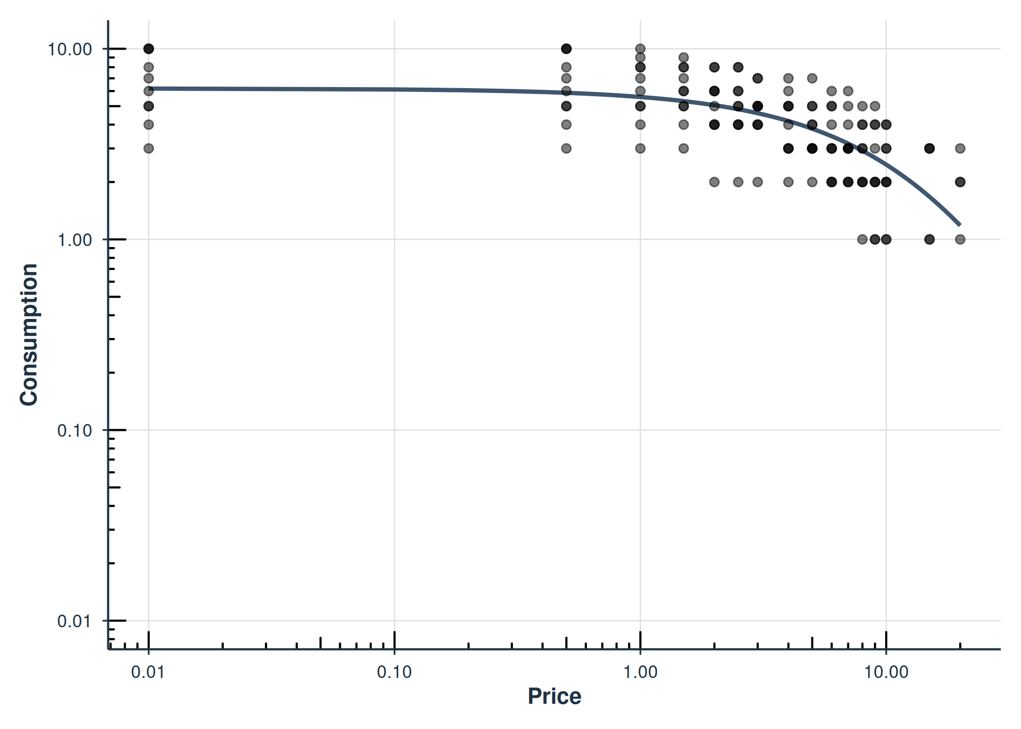
Conclusion
The fit_demand_fixed() interface provides a modern,
consistent API for individual demand curve fitting with full support for
the tidy() / glance() / augment()
workflow. For datasets where borrowing strength across subjects is
desirable, consider the mixed-effects or hurdle model approaches.
See Also
-
vignette("beezdemand")– Getting started with beezdemand -
vignette("model-selection")– Choosing the right model class -
vignette("group-comparisons")– Extra sum-of-squares F-test for group comparisons -
vignette("mixed-demand")– Mixed-effects nonlinear demand models (NLME) -
vignette("mixed-demand-advanced")– Advanced mixed-effects topics -
vignette("hurdle-demand-models")– Two-part hurdle demand models via TMB -
vignette("cross-price-models")– Cross-price demand analysis -
vignette("migration-guide")– Migrating fromFitCurves()tofit_demand_fixed()