Mixed-Effects Demand Modeling with `beezdemand`

Introduction

This vignette demonstrates how to perform mixed-effects nonlinear modeling of behavioral economic demand data using the beezdemand package. We will focus on the fit_demand_mixed() function and its associated helper functions for extracting results, making predictions, and visualizing fits. These models allow for individual differences (random effects) and the examination of how various factors (fixed effects) influence demand parameters like Q_{0} (maximum consumption at zero price) and \alpha (sensitivity of demand to price). The parameters Q_{0} and \alpha are estimated on a log10 scale for numerical stability, but reporting functions will provide them on their natural, interpretable scale.

For advanced topics including multi-factor models, collapsing factor levels, estimated marginal means, pairwise comparisons, continuous covariates, and complex random effects structures, see vignette("mixed-demand-advanced").

Data Preparation

For these examples, we will use the apt and ko datasets, which is assumed to be available and pre-processed.

The apt dataset should contain:

id: A unique identifier for each subject.
x: The price of the drug.
y: The consumption of the drug.

The ko dataset should contain:

monkey: A subject or group identifier for random effects.
x: The price of the commodity (in this case the fixed-ratio requirement).
y: Raw consumption values. This is typically used with the simplified exponentiated equation.
y_ll4: Consumption, ll4 transformed. This is typically used with the zben equation.
Factor columns like drug and dose.

quick_nlme_control <- nlme::nlmeControl(
  msMaxIter = 100,
  niterEM = 20,
  maxIter = 100, # Low iterations for speed
  pnlsTol = 0.1,
  tolerance = 1e-4, # Looser tolerance
  opt = "nlminb",
  msVerbose = FALSE
)

Fitting Demand Models with fit_demand_mixed()

The core function for fitting nonlinear mixed-effects demand models is fit_demand_mixed().

APT Fit and Plot

LL4 transformation with ZBEn

apt_ll4 <- apt |>
  mutate(y_ll4 = ll4(y))

fit_apt_zben <- fit_demand_mixed(
  data = apt_ll4,
  y_var = "y_ll4",
  x_var = "x",
  id_var = "id",
  equation_form = "zben",
  nlme_control = quick_nlme_control,
  start_value_method = "heuristic"
)
print(fit_apt_zben)
#> Demand NLME Model Fit ('beezdemand_nlme' object)
#> ---------------------------------------------------
#> 
#> Call:
#> fit_demand_mixed(data = apt_ll4, y_var = "y_ll4", x_var = "x", 
#>     id_var = "id", equation_form = "zben", start_value_method = "heuristic", 
#>     nlme_control = quick_nlme_control)
#> 
#> Equation Form Selected:  zben 
#> NLME Model Formula:
#> y_ll4 ~ Q0 * exp(-(10^alpha/Q0) * (10^Q0) * x)
#> <environment: 0x55fd24df19b0>
#> Fixed Effects Structure (Q0 & alpha):  ~ 1 
#> Factors: None
#> ID Variable for Random Effects:  id 
#> 
#> Start Values Used (Fixed Effects Intercepts):
#>   Q0 Intercept (log10 scale):  0.8117 
#>   alpha Intercept (log10 scale):  -3 
#> 
#> --- NLME Model Fit Summary (from nlme object) ---
#> Nonlinear mixed-effects model fit by maximum likelihood
#>   Model: nlme_model_formula_obj 
#>   Data: data 
#>   Log-likelihood: 146.7928
#>   Fixed: list(Q0 ~ 1, alpha ~ 1) 
#>         Q0      alpha 
#>  0.8578019 -1.9749801 
#> 
#> Random effects:
#>  Formula: list(Q0 ~ 1, alpha ~ 1)
#>  Level: id
#>  Structure: Diagonal
#>                Q0     alpha   Residual
#> StdDev: 0.1691518 0.2287771 0.07914016
#> 
#> Number of Observations: 160
#> Number of Groups: 10 
#> 
#> --- Additional Fit Statistics ---
#> Log-likelihood:  146.8 
#> AIC:  -283.6 
#> BIC:  -268.2 
#> ---------------------------------------------------

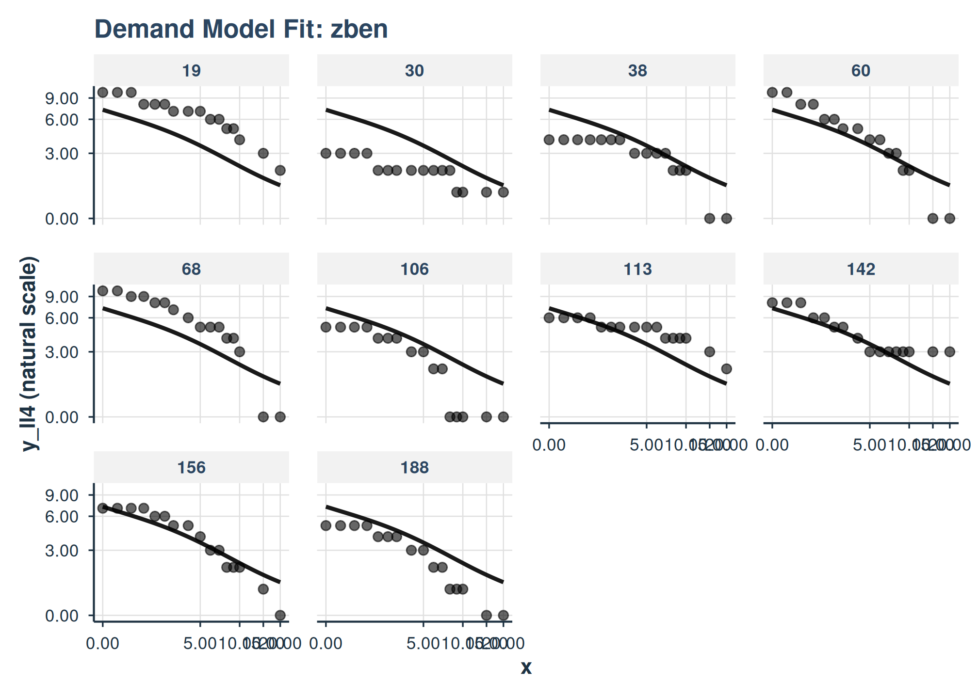
plot(
  fit_apt_zben,
  inv_fun = ll4_inv,
  y_trans = "pseudo_log",
  x_trans = "pseudo_log",
  show_pred_lines = c("population", "individual")
) +
  facet_wrap(
    ~id
  )

Simplified Exponential

fit_apt_simplified <- fit_demand_mixed(
  data = apt_ll4,
  y_var = "y",
  x_var = "x",
  id_var = "id",
  equation_form = "simplified",
  nlme_control = quick_nlme_control,
  start_value_method = "heuristic"
)
print(fit_apt_simplified)
#> Demand NLME Model Fit ('beezdemand_nlme' object)
#> ---------------------------------------------------
#> 
#> Call:
#> fit_demand_mixed(data = apt_ll4, y_var = "y", x_var = "x", id_var = "id", 
#>     equation_form = "simplified", start_value_method = "heuristic", 
#>     nlme_control = quick_nlme_control)
#> 
#> Equation Form Selected:  simplified 
#> NLME Model Formula:
#> y ~ (10^Q0) * exp(-(10^alpha) * (10^Q0) * x)
#> <environment: 0x55fd1bb069e8>
#> Fixed Effects Structure (Q0 & alpha):  ~ 1 
#> Factors: None
#> ID Variable for Random Effects:  id 
#> 
#> Start Values Used (Fixed Effects Intercepts):
#>   Q0 Intercept (log10 scale):  0.8129 
#>   alpha Intercept (log10 scale):  -3 
#> 
#> --- NLME Model Fit Summary (from nlme object) ---
#> Nonlinear mixed-effects model fit by maximum likelihood
#>   Model: nlme_model_formula_obj 
#>   Data: data 
#>   Log-likelihood: -172.7978
#>   Fixed: list(Q0 ~ 1, alpha ~ 1) 
#>         Q0      alpha 
#>  0.8218145 -1.7748511 
#> 
#> Random effects:
#>  Formula: list(Q0 ~ 1, alpha ~ 1)
#>  Level: id
#>  Structure: Diagonal
#>                Q0     alpha  Residual
#> StdDev: 0.1626688 0.1969346 0.5590275
#> 
#> Number of Observations: 160
#> Number of Groups: 10 
#> 
#> --- Additional Fit Statistics ---
#> Log-likelihood:  -172.8 
#> AIC:  355.6 
#> BIC:  371 
#> ---------------------------------------------------

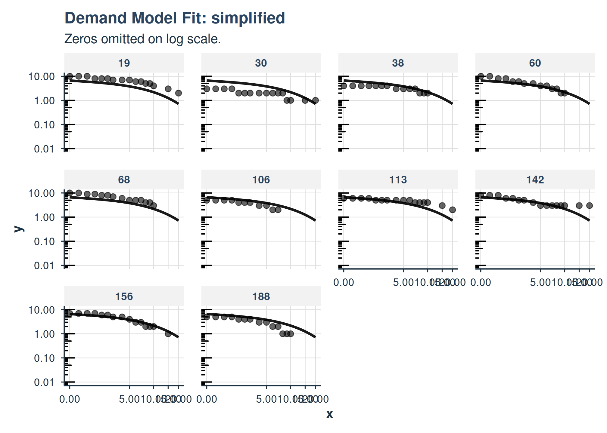
plot(
  fit_apt_simplified,
  x_trans = "pseudo_log",
  show_pred_lines = c("population", "individual")
) +
  facet_wrap(
    ~id
  )

Koffarnus (Exponentiated) Equation Form

fit_demand_mixed() also supports the Koffarnus et al. (2015) equation via equation_form = "exponentiated". By default, the scaling constant k will be computed from the data range (you can also specify it directly).

fit_apt_exponentiated <- fit_demand_mixed(
  data = apt,
  y_var = "y",
  x_var = "x",
  id_var = "id",
  equation_form = "exponentiated",
  k = NULL,
  nlme_control = quick_nlme_control,
  start_value_method = "heuristic"
)
print(fit_apt_exponentiated)
#> Demand NLME Model Fit ('beezdemand_nlme' object)
#> ---------------------------------------------------
#> 
#> Call:
#> fit_demand_mixed(data = apt, y_var = "y", x_var = "x", id_var = "id", 
#>     equation_form = "exponentiated", k = NULL, start_value_method = "heuristic", 
#>     nlme_control = quick_nlme_control)
#> 
#> Equation Form Selected:  exponentiated 
#> NLME Model Formula:
#> y ~ (10^Q0) * 10^(1.5 * (exp(-(10^alpha) * (10^Q0) * x) - 1))
#> <environment: 0x55fd215fde60>
#> Fixed Effects Structure (Q0 & alpha):  ~ 1 
#> Factors: None
#> ID Variable for Random Effects:  id 
#> 
#> Start Values Used (Fixed Effects Intercepts):
#>   Q0 Intercept (log10 scale):  0.8129 
#>   alpha Intercept (log10 scale):  -3 
#> 
#> --- NLME Model Fit Summary (from nlme object) ---
#> Nonlinear mixed-effects model fit by maximum likelihood
#>   Model: nlme_model_formula_obj 
#>   Data: data 
#>   Log-likelihood: -181.3817
#>   Fixed: list(Q0 ~ 1, alpha ~ 1) 
#>         Q0      alpha 
#>  0.8334103 -2.2391878 
#> 
#> Random effects:
#>  Formula: list(Q0 ~ 1, alpha ~ 1)
#>  Level: id
#>  Structure: Diagonal
#>                Q0     alpha  Residual
#> StdDev: 0.1648661 0.2001946 0.5988898
#> 
#> Number of Observations: 160
#> Number of Groups: 10 
#> 
#> --- Additional Fit Statistics ---
#> Log-likelihood:  -181.4 
#> AIC:  372.8 
#> BIC:  388.1 
#> ---------------------------------------------------

Inspecting Fits (tidy / glance / augment)

All modern model classes support tidy(), glance(), and augment() to standardize programmatic access to estimates, model summaries, and residuals.

glance(fit_apt_zben)
#> # A tibble: 1 × 10
#>   model_class     backend equation_form  nobs n_subjects converged logLik   AIC
#>   <chr>           <chr>   <chr>         <int>      <int> <lgl>      <dbl> <dbl>
#> 1 beezdemand_nlme nlme    zben            160         10 TRUE        147. -284.
#> # ℹ 2 more variables: BIC <dbl>, sigma <dbl>
tidy(fit_apt_zben) |> head()
#> # A tibble: 5 × 9
#>   term     estimate std.error statistic   p.value component estimate_scale
#>   <chr>       <dbl>     <dbl>     <dbl>     <dbl> <chr>     <chr>         
#> 1 Q0        7.21      0.919        7.85  4.29e-15 fixed     natural       
#> 2 alpha     0.0106    0.00182      5.83  5.69e- 9 fixed     natural       
#> 3 Q0        0.0286   NA           NA    NA        variance  natural       
#> 4 alpha     0.0523   NA           NA    NA        variance  natural       
#> 5 Residual  0.00626  NA           NA    NA        variance  natural       
#> # ℹ 2 more variables: term_display <chr>, estimate_internal <dbl>
augment(fit_apt_zben) |> head()
#> # A tibble: 6 × 7
#>   id        x     y y_ll4 .fitted   .resid .fixed
#>   <fct> <dbl> <dbl> <dbl>   <dbl>    <dbl>  <dbl>
#> 1 19      0      10 1.00    1.02  -0.0195   0.858
#> 2 19      0.5    10 1.00    0.994  0.00585  0.820
#> 3 19      1      10 1.00    0.969  0.0305   0.785
#> 4 19      1.5     8 0.903   0.945 -0.0423   0.751
#> 5 19      2       8 0.903   0.922 -0.0188   0.718
#> 6 19      2.5     8 0.903   0.899  0.00413  0.687

Diagnostics

Use check_demand_model() and the residual plotting helpers as standard post-fit checks.

check_demand_model(fit_apt_zben)
#> 
#> Model Diagnostics
#> ================================================== 
#> Model class: beezdemand_nlme 
#> 
#> Convergence:
#>   Status: Converged
#> 
#> Random Effects:
#>   Q0 variance: 0.02861
#>   alpha variance: 0.05234
#> 
#> Residuals:
#>   Mean: -0.06639
#>   SD: 0.9396
#>   Range: [-3.621, 2.686]
#>   Outliers: 1 observations
#> 
#> --------------------------------------------------
#> Issues Detected (1):
#>   1. Detected 1 potential outliers (|resid| > 3 SD)
#> 
#> Recommendations:
#>   - Investigate outlying observations
plot_residuals(fit_apt_zben)$fitted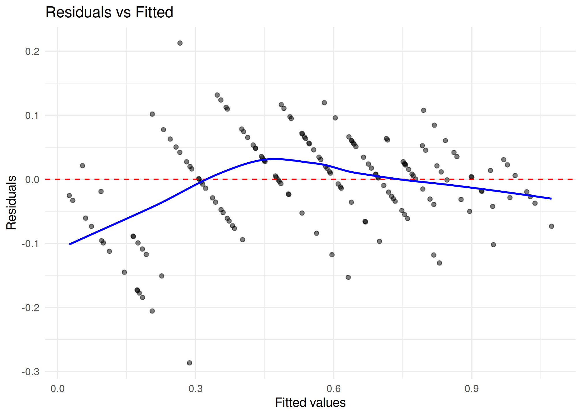

Basic Model (No Factors)

This model estimates global Q_{0} and \alpha parameters with random effects for subjects.

# Make sure a similar 'fit_no_factors' was created successfully in your environment
# For the vignette, let's create one that is more likely to converge quickly
# by using only Alfentanil data, which is less complex than the full dataset.
ko_alf <- ko[ko$drug == "Alfentanil", ]

fit_no_factors_vignette <- fit_demand_mixed(
  data = ko_alf,
  y_var = "y_ll4",
  x_var = "x",
  id_var = "monkey",
  equation_form = "zben",
  nlme_control = quick_nlme_control, # Use quicker control for vignette
  start_value_method = "heuristic" # Heuristic is faster for simple model
)
print(fit_no_factors_vignette)
#> Demand NLME Model Fit ('beezdemand_nlme' object)
#> ---------------------------------------------------
#> 
#> Call:
#> fit_demand_mixed(data = ko_alf, y_var = "y_ll4", x_var = "x", 
#>     id_var = "monkey", equation_form = "zben", start_value_method = "heuristic", 
#>     nlme_control = quick_nlme_control)
#> 
#> Equation Form Selected:  zben 
#> NLME Model Formula:
#> y_ll4 ~ Q0 * exp(-(10^alpha/Q0) * (10^Q0) * x)
#> <environment: 0x55fd1fc87758>
#> Fixed Effects Structure (Q0 & alpha):  ~ 1 
#> Factors: None
#> ID Variable for Random Effects:  monkey 
#> 
#> Start Values Used (Fixed Effects Intercepts):
#>   Q0 Intercept (log10 scale):  2.271 
#>   alpha Intercept (log10 scale):  -3 
#> 
#> --- NLME Model Fit Summary (from nlme object) ---
#> Nonlinear mixed-effects model fit by maximum likelihood
#>   Model: nlme_model_formula_obj 
#>   Data: data 
#>   Log-likelihood: 2.763668
#>   Fixed: list(Q0 ~ 1, alpha ~ 1) 
#>        Q0     alpha 
#>  2.131113 -4.665222 
#> 
#> Random effects:
#>  Formula: list(Q0 ~ 1, alpha ~ 1)
#>  Level: monkey
#>  Structure: Diagonal
#>                   Q0        alpha  Residual
#> StdDev: 5.264342e-06 3.217971e-06 0.2275573
#> 
#> Number of Observations: 45
#> Number of Groups: 3 
#> 
#> --- Additional Fit Statistics ---
#> Log-likelihood:  2.764 
#> AIC:  4.473 
#> BIC:  13.51 
#> ---------------------------------------------------

The output shows the model call, selected equation form, and if the model converged, it prints the nlme model summary.

Model with One Factor

Let’s model Q_{0} and \alpha as varying by dose for Alfentanil.

fit_one_factor_dose <- fit_demand_mixed(
  data = ko_alf,
  y_var = "y_ll4",
  x_var = "x",
  id_var = "monkey",
  factors = "dose",
  equation_form = "zben",
  nlme_control = quick_nlme_control,
  start_value_method = "heuristic"
)
print(fit_one_factor_dose)
#> Demand NLME Model Fit ('beezdemand_nlme' object)
#> ---------------------------------------------------
#> 
#> Call:
#> fit_demand_mixed(data = ko_alf, y_var = "y_ll4", x_var = "x", 
#>     id_var = "monkey", factors = "dose", equation_form = "zben", 
#>     start_value_method = "heuristic", nlme_control = quick_nlme_control)
#> 
#> Equation Form Selected:  zben 
#> NLME Model Formula:
#> y_ll4 ~ Q0 * exp(-(10^alpha/Q0) * (10^Q0) * x)
#> <environment: 0x55fd20f00628>
#> Fixed Effects Structure (Q0 & alpha):  ~ dose 
#> Factors:  dose 
#> Interaction Term Included:  FALSE 
#> ID Variable for Random Effects:  monkey 
#> 
#> Start Values Used (Fixed Effects Intercepts):
#>   Q0 Intercept (log10 scale):  2.271 
#>   alpha Intercept (log10 scale):  -3 
#> 
#> --- NLME Model Fit Summary (from nlme object) ---
#> Nonlinear mixed-effects model fit by maximum likelihood
#>   Model: nlme_model_formula_obj 
#>   Data: data 
#>   Log-likelihood: 17.90035
#>   Fixed: list(Q0 ~ dose, alpha ~ dose) 
#>    Q0.(Intercept)      Q0.dose0.001      Q0.dose0.003 alpha.(Intercept) 
#>       2.415349697      -0.257733998      -0.519065274      -4.650854662 
#>   alpha.dose0.001   alpha.dose0.003 
#>      -0.084081282       0.009734048 
#> 
#> Random effects:
#>  Formula: list(Q0 ~ 1, alpha ~ 1)
#>  Level: monkey
#>  Structure: Diagonal
#>         Q0.(Intercept) alpha.(Intercept)  Residual
#> StdDev:   3.760034e-06      2.301156e-06 0.1625574
#> 
#> Number of Observations: 45
#> Number of Groups: 3 
#> 
#> --- Additional Fit Statistics ---
#> Log-likelihood:  17.9 
#> AIC:  -17.8 
#> BIC:  -1.541 
#> ---------------------------------------------------

Inspecting Model Fits

Once a model is fit, you can inspect it using several S3 methods.

# Summary
summary(fit_one_factor_dose)
#> 
#> Nonlinear Mixed-Effects Demand Model Summary
#> ================================================== 
#> 
#> Model Specification:
#>   Equation form: zben 
#>   Factors: dose 
#>   Interaction: FALSE 
#>   ID variable: monkey 
#> 
#> Data Summary:
#>   Subjects: 3 
#>   Observations: 45 
#> 
#> Fixed Effects:
#>                       Value Std.Error        DF t-value  p-value    
#> Q0.(Intercept)    2.602e+02 4.474e+01 3.700e+01   5.817 5.99e-09 ***
#> Q0.dose0.001      5.524e-01 1.264e-01 3.700e+01   4.370 1.24e-05 ***
#> Q0.dose0.003      3.026e-01 6.833e-02 3.700e+01   4.429 9.46e-06 ***
#> alpha.(Intercept) 2.234e-05 2.695e-06 3.700e+01   8.289  < 2e-16 ***
#> alpha.dose0.001   8.240e-01 1.387e-01 3.700e+01   5.941 2.84e-09 ***
#> alpha.dose0.003   1.023e+00 1.792e-01 3.700e+01   5.707 1.15e-08 ***
#> ---
#> Signif. codes:  0 '***' 0.001 '**' 0.01 '*' 0.05 '.' 0.1 ' ' 1
#> 
#> Random Effects:
#> monkey = pdDiag(list(Q0 ~ 1,alpha ~ 1)) 
#>                   Variance     StdDev      
#> Q0.(Intercept)    1.413786e-11 3.760034e-06
#> alpha.(Intercept) 5.295319e-12 2.301156e-06
#> Residual          2.642491e-02 1.625574e-01
#> 
#> Residual standard error: 0.1626 
#> 
#> Model Fit:
#>   Log-Likelihood: 17.9 
#>   AIC: -17.8 
#>   BIC: -1.54

# Fixed effects
coef(fit_one_factor_dose, type = "fixed")
#>    Q0.(Intercept)      Q0.dose0.001      Q0.dose0.003 alpha.(Intercept) 
#>       2.415349697      -0.257733998      -0.519065274      -4.650854662 
#>   alpha.dose0.001   alpha.dose0.003 
#>      -0.084081282       0.009734048

# Random effects (deviations from fixed)
head(coef(fit_one_factor_dose, type = "random"))
#>   Q0.(Intercept) alpha.(Intercept)
#> A   8.830297e-11     -3.424853e-10
#> B   1.246265e-10      3.352306e-11
#> C  -2.129295e-10      3.089622e-10

# Subject-specific coefficients (fixed + random)
head(coef(fit_one_factor_dose, type = "combined"))
#>   Q0.(Intercept) Q0.dose0.001 Q0.dose0.003 alpha.(Intercept) alpha.dose0.001
#> A        2.41535    -0.257734   -0.5190653         -4.650855     -0.08408128
#> B        2.41535    -0.257734   -0.5190653         -4.650855     -0.08408128
#> C        2.41535    -0.257734   -0.5190653         -4.650855     -0.08408128
#>   alpha.dose0.003
#> A     0.009734048
#> B     0.009734048
#> C     0.009734048

# Access nlme fixef/ranef directly
nlme::fixef(fit_one_factor_dose)
#>    Q0.(Intercept)      Q0.dose0.001      Q0.dose0.003 alpha.(Intercept) 
#>       2.415349697      -0.257733998      -0.519065274      -4.650854662 
#>   alpha.dose0.001   alpha.dose0.003 
#>      -0.084081282       0.009734048
utils::head(nlme::ranef(fit_one_factor_dose))
#>   Q0.(Intercept) alpha.(Intercept)
#> A   8.830297e-11     -3.424853e-10
#> B   1.246265e-10      3.352306e-11
#> C  -2.129295e-10      3.089622e-10

# Start values that were used for the NLME fit
fit_one_factor_dose$start_values_used
#> [1]  2.270679  0.000000  0.000000 -3.000000  0.000000  0.000000

Making Predictions (predict())

The S3 predict() method can generate population-level or group-level predictions.

# Population-level predictions (log10 scale for 'zben')
preds_pop_log <- predict(fit_one_factor_dose, level = 0)
head(preds_pop_log)
#> # A tibble: 6 × 7
#>   monkey     x     y y_ll4 drug       dose  .fitted
#>   <fct>  <dbl> <dbl> <dbl> <fct>      <fct>   <dbl>
#> 1 A         10 120.  2.08  Alfentanil 0.003   1.88 
#> 2 A         32 110   2.04  Alfentanil 0.003   1.84 
#> 3 A        100  66.5 1.82  Alfentanil 0.003   1.72 
#> 4 A        320  39   1.59  Alfentanil 0.003   1.40 
#> 5 A       1000   9.5 0.978 Alfentanil 0.003   0.734
#> 6 B         10  77   1.89  Alfentanil 0.003   1.88

# Population-level predictions (natural scale, back-transformed)
preds_pop_natural <- predict(
  fit_one_factor_dose,
  level = 0,
  inv_fun = ll4_inv
)
head(preds_pop_natural)
#> # A tibble: 6 × 7
#>   monkey     x     y y_ll4 drug       dose  .fitted
#>   <fct>  <dbl> <dbl> <dbl> <fct>      <fct>   <dbl>
#> 1 A         10 120.  2.08  Alfentanil 0.003   75.6 
#> 2 A         32 110   2.04  Alfentanil 0.003   69.1 
#> 3 A        100  66.5 1.82  Alfentanil 0.003   53.0 
#> 4 A        320  39   1.59  Alfentanil 0.003   25.1 
#> 5 A       1000   9.5 0.978 Alfentanil 0.003    5.42
#> 6 B         10  77   1.89  Alfentanil 0.003   75.6

# Group-level predictions for first few data points
sample_newdata <- fit_one_factor_dose$data[1:5, ]
preds_group_log <- predict(fit_one_factor_dose, newdata = sample_newdata, level = 1)
preds_group_log
#> # A tibble: 5 × 7
#>   monkey     x     y y_ll4 drug       dose  .fitted
#>   <fct>  <dbl> <dbl> <dbl> <fct>      <fct>   <dbl>
#> 1 A         10 120.  2.08  Alfentanil 0.003   1.88 
#> 2 A         32 110   2.04  Alfentanil 0.003   1.84 
#> 3 A        100  66.5 1.82  Alfentanil 0.003   1.72 
#> 4 A        320  39   1.59  Alfentanil 0.003   1.40 
#> 5 A       1000   9.5 0.978 Alfentanil 0.003   0.734

Visualizing Model Fits with `plot()`

The beezdemand package provides an S3 plot() method for beezdemand_nlme objects, built using ggplot2, to help visualize the fitted demand curves against observed data.

Key Features:

Observed Data: Can display the original data points.
Prediction Lines: Plots model-predicted demand curves at the population level (fixed effects, pred_level = 0) or group/subject level (fixed + random effects, pred_level = 1).
Inverse Transformation (inv_fun): Allows back-transformation of the y-axis and predictions to the natural scale (e.g., from log10 consumption back to raw consumption units).
Aesthetic Mapping: Factors can be mapped to color, linetype (for lines), and shape (for points).
Faceting: Supports ggplot2 faceting via facet_formula.
Axis Transformations: Allows x_trans and y_trans (e.g., “log10”, “pseudo_log”).

Example 1: Plotting a Single-Factor Model

Let’s use fit_one_factor_dose (modeling demand for Alfentanil by dose, with y_ll4 as the dependent variable).

plot(
  fit_one_factor_dose,
  inv_fun = ll4_inv,
  color_by = "dose",
  shape_by = "dose",
  observed_point_alpha = 0.7,
  title = "Alfentanil Demand by Dose (Population Fit)"
)

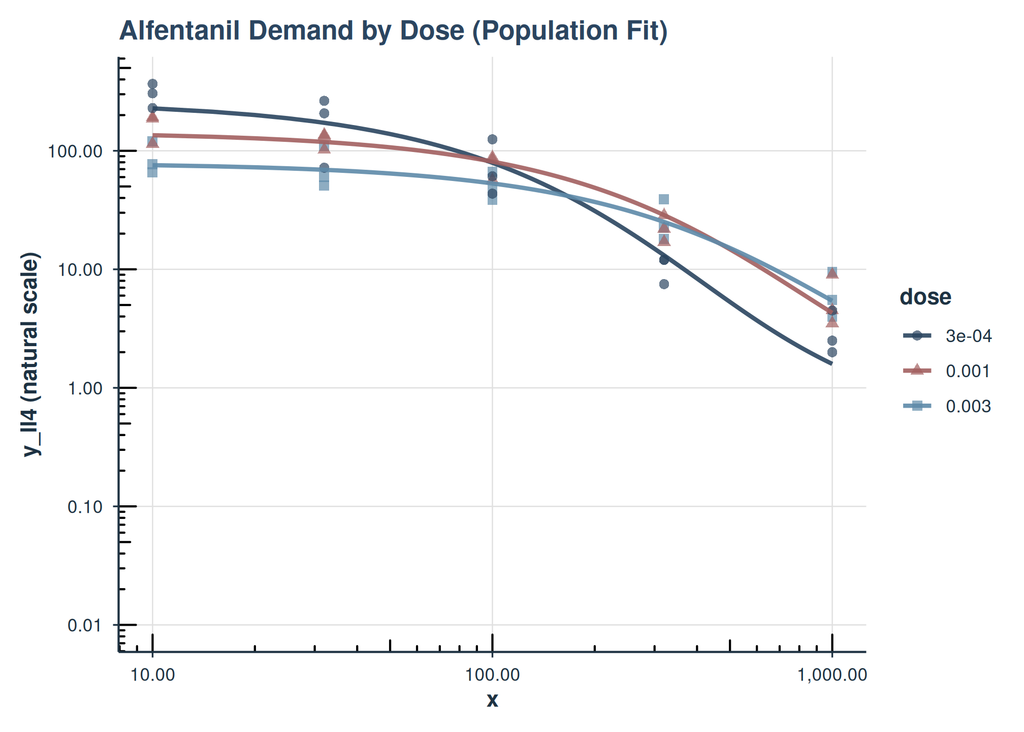
Demand curves for Alfentanil by dose (population level). y-axis on natural scale.

This plot shows the population-level demand curves for each dose of Alfentanil. The y-axis has been back-transformed to the natural consumption scale using inv_fun.

Example 2: Plotting Subject-Specific Lines

We can also visualize the individual subject fits by setting show_pred_lines = "individual".

plot(
  fit_one_factor_dose,
  show_pred_lines = "individual",
  inv_fun = ll4_inv,
  color_by = "dose",
  observed_point_alpha = 0.4,
  y_trans = "pseudo_log",
  ind_line_alpha = .5,
  title = "Alfentanil Demand by Dose (Subject-Specific Fits)"
) +
  ggplot2::guides(color = guide_legend(override.aes = list(alpha = 1))) +
  facet_grid(~monkey)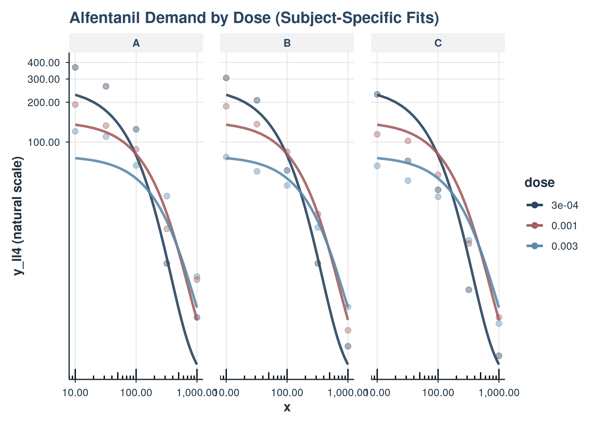

Here, each thin line represents the fitted curve for an individual subject (monkey), colored by dose.

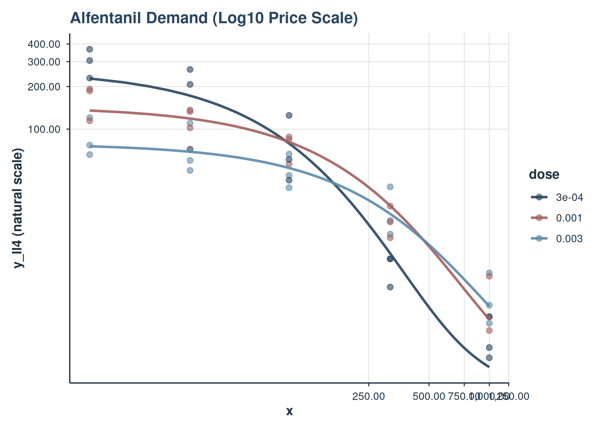
Example 3: Customizing Axes (e.g., Log Scale)

You can use x_trans and y_trans for axis transformations.

plot(
  fit_one_factor_dose,
  inv_fun = ll4_inv,
  color_by = "dose",
  x_trans = "pseudo_log",
  y_trans = "pseudo_log",
  title = "Alfentanil Demand (Log10 Price Scale)"
)

Users can further customize the returned ggplot object by adding more layers or theme adjustments. For instance, to add custom axis limits or breaks:

plot_object +
    ggplot2::scale_x_continuous(
        limits = c(0, 1000),
        breaks = c(0, 100, 500, 1000)
    )

Conclusion

The beezdemand package provides a suite of tools for robustly fitting nonlinear mixed-effects demand models and interpreting their parameters. By parameterizing Q_{0} and \alpha on the log10 scale, numerical stability is enhanced, while helper functions allow for easy back-transformation and interpretation on the natural scale.

Brent Kaplan

2026-03-03

Introduction

Data Preparation

Fitting Demand Models with fit_demand_mixed()

APT Fit and Plot

LL4 transformation with ZBEn

Simplified Exponential

Koffarnus (Exponentiated) Equation Form

Inspecting Fits (tidy / glance / augment)

Diagnostics

Basic Model (No Factors)

Model with One Factor

Inspecting Model Fits

Making Predictions (predict())

Visualizing Model Fits with `plot()`

Example 1: Plotting a Single-Factor Model

Example 2: Plotting Subject-Specific Lines

Example 3: Customizing Axes (e.g., Log Scale)

Conclusion

See Also

Mixed-Effects Demand Modeling with `beezdemand`

Brent Kaplan

2026-03-03

Introduction

Data Preparation

Fitting Demand Models with fit_demand_mixed()

APT Fit and Plot

LL4 transformation with ZBEn

Simplified Exponential

Koffarnus (Exponentiated) Equation Form

Inspecting Fits (tidy / glance / augment)

Diagnostics

Basic Model (No Factors)

Model with One Factor

Inspecting Model Fits

Making Predictions (predict())

Visualizing Model Fits with plot()

Example 1: Plotting a Single-Factor Model

Example 2: Plotting Subject-Specific Lines

Example 3: Customizing Axes (e.g., Log Scale)

Conclusion

See Also

Visualizing Model Fits with `plot()`