Advanced Mixed-Effects Demand Modeling

Introduction

This vignette covers advanced topics for mixed-effects nonlinear demand modeling with beezdemand. It assumes you are already familiar with the basics covered in vignette("mixed-demand"), including fitting models with fit_demand_mixed(), inspecting results with tidy() / glance() / augment(), and basic plotting.

Topics covered here include:

Multi-factor models (additive and interaction)
Collapsing factor levels (asymmetric specifications for Q0 and alpha)
Estimated marginal means and pairwise comparisons
Multi-factor visualization with faceting
Complex random effects structures
Continuous covariates and fixed_rhs
Trends with emtrends

quick_nlme_control <- nlme::nlmeControl(
  msMaxIter = 100,
  niterEM = 20,
  maxIter = 100, # Low iterations for speed
  pnlsTol = 0.1,
  tolerance = 1e-4, # Looser tolerance
  opt = "nlminb",
  msVerbose = FALSE
)

# Prepare data subsets used throughout
ko_alf <- ko[ko$drug == "Alfentanil", ]

# Fit the one-factor model used as a baseline/fallback in later sections
fit_one_factor_dose <- fit_demand_mixed(
  data = ko_alf,
  y_var = "y_ll4",
  x_var = "x",
  id_var = "monkey",
  factors = "dose",
  equation_form = "zben",
  nlme_control = quick_nlme_control,
  start_value_method = "heuristic"
)

Model with Two Factors (Additive)

Here, Q_{0} and \alpha vary by drug and dose additively. For this, we need more data than just ko_alf, so we use ko. Note: With complex models and small sample sizes, convergence can be challenging. The start_value_method = “pooled_nls” is often more robust for complex models.

This example is computationally intensive and is not run during standard vignette building. To run it, set BEEZDEMAND_VIGNETTE_MODE=full as an environment variable before building. When successful, the output shows fixed-effect estimates for each drug and dose combination on Q0 and alpha, plus random-effects variance components.

Model with Two Factors and Interaction

This allows the effect of dose to be different for each drug (and vice-versa).

This example is computationally intensive and is not run during standard vignette building. The interaction model allows the effect of dose to differ by drug (and vice versa), producing drug:dose interaction terms in the fixed-effects table.

Using Different equation_form and y_var

The simplified equation form expects y_var to be raw consumption.

This example uses equation_form = "simplified" with raw consumption values (no LL4 transformation needed). The simplified equation handles zeros natively. When this example runs, the output resembles the zben model output but with y as the dependent variable.

Collapsing Factor Levels

Sometimes you might want to group levels of a factor, and you may want different groupings for Q_{0} versus \alpha. The collapse_levels argument allows you to specify separate collapsing schemes for each parameter.

Structure:

collapse_levels = list(
  Q0 = list(factor_name = list(new_level = c("old_level1", "old_level2"), ...)),
  alpha = list(factor_name = list(new_level = c("old_level1", ...), ...))
)

Either Q0 or alpha (or both) can be omitted to keep original levels for that parameter.

Example: Same collapsing for both parameters

# Ensure levels to collapse are present in ko_alf$dose
# levels(ko_alf$dose) are "0.001", "0.003", "3e-04"
fit_collapsed_same <- try(
  fit_demand_mixed(
    data = ko_alf,
    y_var = "y_ll4",
    x_var = "x",
    id_var = "monkey",
    factors = "dose",
    collapse_levels = list(
      Q0 = list(
        dose = list(low_doses = c("3e-04", "0.001"), high_dose = "0.003")
      ),
      alpha = list(
        dose = list(low_doses = c("3e-04", "0.001"), high_dose = "0.003")
      )
    ),
    equation_form = "zben",
    nlme_control = quick_nlme_control
  ),
  silent = TRUE
)

if (
  !is.null(fit_collapsed_same) &&
    !inherits(fit_collapsed_same, "try-error") &&
    !is.null(fit_collapsed_same$model)
) {
  print(fit_collapsed_same)
  cat("\nQ0 params:", fit_collapsed_same$param_info$num_params_Q0, "\n")
  cat("alpha params:", fit_collapsed_same$param_info$num_params_alpha, "\n")
} else {
  cat("Collapsed levels model failed to converge.\n")
}
#> Demand NLME Model Fit ('beezdemand_nlme' object)
#> ---------------------------------------------------
#> 
#> Call:
#> fit_demand_mixed(data = ko_alf, y_var = "y_ll4", x_var = "x", 
#>     id_var = "monkey", factors = "dose", equation_form = "zben", 
#>     collapse_levels = list(Q0 = list(dose = list(low_doses = c("3e-04", 
#>         "0.001"), high_dose = "0.003")), alpha = list(dose = list(low_doses = c("3e-04", 
#>         "0.001"), high_dose = "0.003"))), nlme_control = quick_nlme_control)
#> 
#> Equation Form Selected:  zben 
#> NLME Model Formula:
#> y_ll4 ~ Q0 * exp(-(10^alpha/Q0) * (10^Q0) * x)
#> <environment: 0x55b798538b98>
#> Fixed Effects Structure (Q0):     ~ dose_Q0 
#> Fixed Effects Structure (alpha):  ~ dose_alpha 
#> Factors:  dose 
#> Interaction Term Included:  FALSE 
#> ID Variable for Random Effects:  monkey 
#> 
#> Start Values Used (Fixed Effects Intercepts):
#>   Q0 Intercept (log10 scale):  2.271 
#>   alpha Intercept (log10 scale):  -3 
#> 
#> --- NLME Model Fit Summary (from nlme object) ---
#> Nonlinear mixed-effects model fit by maximum likelihood
#>   Model: nlme_model_formula_obj 
#>   Data: data 
#>   Log-likelihood: 10.80738
#>   Fixed: list(Q0 ~ dose_Q0, alpha ~ dose_alpha) 
#>            Q0.(Intercept)       Q0.dose_Q0low_doses         alpha.(Intercept) 
#>                1.89628442                0.37072017               -4.64112061 
#> alpha.dose_alphalow_doses 
#>               -0.04341491 
#> 
#> Random effects:
#>  Formula: list(Q0 ~ 1, alpha ~ 1)
#>  Level: monkey
#>  Structure: Diagonal
#>         Q0.(Intercept) alpha.(Intercept)  Residual
#> StdDev:   4.401177e-06      2.693877e-06 0.1903097
#> 
#> Number of Observations: 45
#> Number of Groups: 3 
#> 
#> --- Additional Fit Statistics ---
#> Log-likelihood:  10.81 
#> AIC:  -7.615 
#> BIC:  5.032 
#> ---------------------------------------------------
#> 
#> Q0 params: 2 
#> alpha params: 2

Example: Different collapsing for Q0 and alpha

This is particularly useful when you want fine-grained distinctions for one parameter but not the other. For instance, you might hypothesize that maximum consumption (Q_{0}) varies by dose, but sensitivity (\alpha) does not.

# Q0: keep 2 collapsed levels (low vs high)
# alpha: collapse all to 1 level (intercept only)
fit_collapsed_asymmetric <- try(
  fit_demand_mixed(
    data = ko_alf,
    y_var = "y_ll4",
    x_var = "x",
    id_var = "monkey",
    factors = "dose",
    collapse_levels = list(
      Q0 = list(
        dose = list(low_doses = c("3e-04", "0.001"), high_dose = "0.003")
      ),
      alpha = list(dose = list(all_doses = c("3e-04", "0.001", "0.003")))
    ),
    equation_form = "zben",
    nlme_control = quick_nlme_control
  ),
  silent = TRUE
)

if (
  !is.null(fit_collapsed_asymmetric) &&
    !inherits(fit_collapsed_asymmetric, "try-error") &&
    !is.null(fit_collapsed_asymmetric$model)
) {
  print(fit_collapsed_asymmetric)
  cat("\nQ0 params:", fit_collapsed_asymmetric$param_info$num_params_Q0, "\n")
  cat(
    "alpha params:",
    fit_collapsed_asymmetric$param_info$num_params_alpha,
    "\n"
  )
  cat(
    "\nQ0 formula:",
    fit_collapsed_asymmetric$formula_details$fixed_effects_formula_str_Q0,
    "\n"
  )
  cat(
    "alpha formula:",
    fit_collapsed_asymmetric$formula_details$fixed_effects_formula_str_alpha,
    "\n"
  )
} else {
  cat("Asymmetric collapsed levels model failed to converge.\n")
}
#> Demand NLME Model Fit ('beezdemand_nlme' object)
#> ---------------------------------------------------
#> 
#> Call:
#> fit_demand_mixed(data = ko_alf, y_var = "y_ll4", x_var = "x", 
#>     id_var = "monkey", factors = "dose", equation_form = "zben", 
#>     collapse_levels = list(Q0 = list(dose = list(low_doses = c("3e-04", 
#>         "0.001"), high_dose = "0.003")), alpha = list(dose = list(all_doses = c("3e-04", 
#>         "0.001", "0.003")))), nlme_control = quick_nlme_control)
#> 
#> Equation Form Selected:  zben 
#> NLME Model Formula:
#> y_ll4 ~ Q0 * exp(-(10^alpha/Q0) * (10^Q0) * x)
#> <environment: 0x55b7972fe000>
#> Fixed Effects Structure (Q0):     ~ dose_Q0 
#> Fixed Effects Structure (alpha):  ~ 1 
#> Factors:  dose 
#> Interaction Term Included:  FALSE 
#> ID Variable for Random Effects:  monkey 
#> 
#> Start Values Used (Fixed Effects Intercepts):
#>   Could not determine Q0/alpha intercepts from start_values_used structure.
#>   Full start_values_used vector:
#> [1]  2.271  0.000 -3.000
#> 
#> --- NLME Model Fit Summary (from nlme object) ---
#> Nonlinear mixed-effects model fit by maximum likelihood
#>   Model: nlme_model_formula_obj 
#>   Data: data 
#>   Log-likelihood: 10.73793
#>   Fixed: list(Q0 ~ dose_Q0, alpha ~ 1) 
#>      Q0.(Intercept) Q0.dose_Q0low_doses               alpha 
#>           1.9041039           0.3572637          -4.6750675 
#> 
#> Random effects:
#>  Formula: list(Q0 ~ 1, alpha ~ 1)
#>  Level: monkey
#>  Structure: Diagonal
#>         Q0.(Intercept)        alpha  Residual
#> StdDev:   4.409119e-06 2.697381e-06 0.1906036
#> 
#> Number of Observations: 45
#> Number of Groups: 3 
#> 
#> --- Additional Fit Statistics ---
#> Log-likelihood:  10.74 
#> AIC:  -9.476 
#> BIC:  1.364 
#> ---------------------------------------------------
#> 
#> Q0 params: 2 
#> alpha params: 1 
#> 
#> Q0 formula: ~ dose_Q0 
#> alpha formula: ~ 1

Note: When all levels of a factor are collapsed to a single level for a parameter, that factor is automatically removed from the formula for that parameter (it contributes only to the intercept). A message will inform you when this occurs.

EMMs and Comparisons with Collapsed Factors

When using collapse_levels, the get_demand_param_emms() and get_demand_comparisons() functions automatically handle the asymmetric factor structures. EMMs will be computed using the collapsed levels, and comparisons will only be performed when there are multiple levels to compare.

Differential Collapsing Output: When Q0 and alpha have different numbers of factor levels (e.g., Q0 keeps original dose levels while alpha collapses to fewer groups), the EMM output will include separate factor columns:

Original factor column (e.g., dose) for the uncollapsed parameter (Q0)
Suffixed column (e.g., dose_alpha) for the collapsed parameter (alpha)

This results in a cross-joined table showing all combinations of Q0 levels and alpha levels. For example, if dose has 5 original levels and alpha collapses to 2 groups, the EMM table will have 10 rows (5 × 2).

# Using the asymmetric collapsed model from above (if it converged)
if (
  !is.null(fit_collapsed_asymmetric) &&
    !inherits(fit_collapsed_asymmetric, "try-error") &&
    !is.null(fit_collapsed_asymmetric$model)
) {
  cat("--- EMMs with collapsed factors ---\n")
  # EMMs will show collapsed Q0 levels but single alpha value
  collapsed_emms <- get_demand_param_emms(
    fit_obj = fit_collapsed_asymmetric,
    factors_in_emm = "dose", # Use original factor name
    include_ev = TRUE
  )
  print(collapsed_emms)

  cat("\n--- Comparisons with collapsed factors ---\n")
  # Q0 will have comparisons (2 levels), alpha will have none (1 level)
  collapsed_comparisons <- get_demand_comparisons(
    fit_obj = fit_collapsed_asymmetric,
    compare_specs = ~dose, # Use original factor name
    params_to_compare = c("Q0", "alpha")
  )

  cat("\nQ0 contrasts (collapsed levels):\n")
  print(collapsed_comparisons$Q0$contrasts_log10)

  cat("\nalpha contrasts (intercept-only, no comparisons):\n")
  print(collapsed_comparisons$alpha$contrasts_log10)
} else {
  cat("Asymmetric collapsed model not available for EMM demonstration.\n")
}
#> --- EMMs with collapsed factors ---
#> # A tibble: 2 × 16
#>   dose      Q0_param_log10 LCL_Q0_param_log10 UCL_Q0_param_log10 Q0_natural
#>   <fct>              <dbl>              <dbl>              <dbl>      <dbl>
#> 1 high_dose           1.90               1.77               2.04       80.2
#> 2 low_doses           2.26               2.16               2.36      183. 
#> # ℹ 11 more variables: LCL_Q0_natural <dbl>, UCL_Q0_natural <dbl>,
#> #   alpha_param_log10 <dbl>, LCL_alpha_param_log10 <dbl>,
#> #   UCL_alpha_param_log10 <dbl>, alpha_natural <dbl>, LCL_alpha_natural <dbl>,
#> #   UCL_alpha_natural <dbl>, EV <dbl>, LCL_EV <dbl>, UCL_EV <dbl>
#> 
#> --- Comparisons with collapsed factors ---
#> 
#> Q0 contrasts (collapsed levels):
#> # A tibble: 1 × 8
#>   contrast_definition   estimate     SE    df lower.CL upper.CL t.ratio  p.value
#>   <chr>                    <dbl>  <dbl> <dbl>    <dbl>    <dbl>   <dbl>    <dbl>
#> 1 high_dose - low_doses   -0.357 0.0803    40   -0.520   -0.195   -4.45  6.73e-5
#> 
#> alpha contrasts (intercept-only, no comparisons):
#> # A tibble: 0 × 0

Visualizing Multi-Factor Models

Plotting a Two-Factor Model with Faceting

Let’s use fit_two_factors_add (if it converged: y_ll4 ~ drug + dose). We can facet by one factor and color by another.

# Assuming fit_two_factors_add was successfully created earlier
# If it failed, this chunk won't produce a plot.
active_two_factor_fit <- if (
  !is.null(fit_two_factors_add) && !is.null(fit_two_factors_add$model)
) {
  fit_two_factors_add
} else {
  # Fallback to a simpler model if the two-factor one failed in the vignette
  if (!is.null(fit_one_factor_dose$model)) fit_one_factor_dose else NULL
}

if (
  !is.null(active_two_factor_fit$model) &&
    !is.null(active_two_factor_fit$param_info$factors) &&
    length(active_two_factor_fit$param_info$factors) >= 1
) {
  # Determine factors for aesthetics based on what's in active_two_factor_fit
  color_factor <- if ("dose" %in% active_two_factor_fit$param_info$factors) {
    "dose"
  } else {
    NULL
  }
  facet_factor_name <- if (
    "drug" %in% active_two_factor_fit$param_info$factors
  ) {
    "drug"
  } else {
    # If only 'dose' is available from fit_one_factor_dose, we can't facet by 'drug'
    # So, maybe facet by dose instead, or don't facet.
    if (
      "dose" %in%
        active_two_factor_fit$param_info$factors &&
        is.null(color_factor)
    ) {
      color_factor <- "dose" # color by dose if not faceting by it
      NULL # No faceting
    } else {
      NULL
    }
  }

  facet_formula_plot <- if (!is.null(facet_factor_name)) {
    stats::as.formula(paste("~", facet_factor_name))
  } else {
    NULL
  }

  plot(
    active_two_factor_fit,
    inv_fun = ll4_inv,
    color_by = color_factor,
    # linetype_by = if("dose" %in% active_two_factor_fit$param_info$factors) "dose" else NULL, # Example
    facet_formula = facet_formula_plot,
    title = "Demand Curves (Population Fit)",
    observed_point_alpha = 0.5,
    ind_line_alpha = .5
  )
} else {
  cat(
    "A suitable two-factor or one-factor model object not available for this plotting example.\n"
  )
}

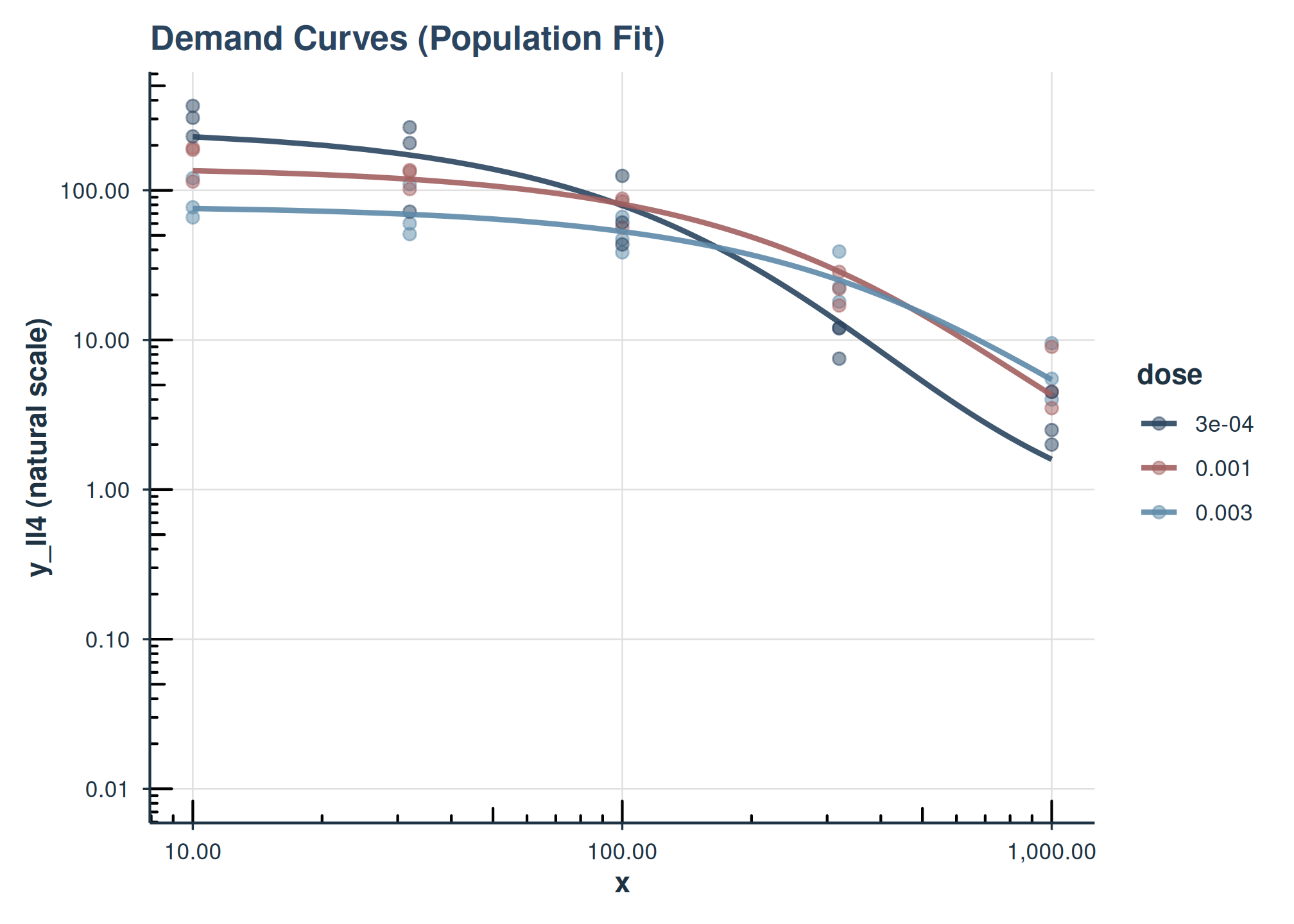
This example attempts to use fit_two_factors_add. If that model didn’t converge (common with minimal iterations for vignette speed), it falls back to fit_one_factor_dose and adjusts aesthetics. The plot will show population lines, colored by one factor and faceted by another (if two factors are available).

Plotting a Model Fit with equation_form = “simplified”

If you fit a model using equation_form = “simplified” (which models raw y), the inv_fun is typically identity because predictions are already on the natural scale.

# Assuming fit_simplified_example converged earlier
if (
  !is.null(fit_simplified_example) && !is.null(fit_simplified_example$model)
) {
  plot(
    fit_simplified_example,
    inv_fun = identity, # Predictions are already on raw y scale
    color_by = "dose",
    shape_by = "dose",
    title = "Demand Model ('simplified' equation, Raw Y)"
  )
} else {
  cat("fit_simplified_example model object not available for plotting.\n")
}
#> fit_simplified_example model object not available for plotting.

Users can further customize the returned ggplot object by adding more layers or theme adjustments. For instance, to add custom axis limits or breaks:

plot_object +
    ggplot2::scale_x_continuous(
        limits = c(0, 1000),
        breaks = c(0, 100, 500, 1000)
    )

Analyzing Estimated Marginal Means (`get_demand_param_emms`)

This function helps interpret how factors affect Q_{0} and \alpha, providing estimates on both log10 and natural scales, and optionally Essential Value (EV).

Note on collapse_levels: When a model is fit using collapse_levels with asymmetric specifications (different collapsing for Q0 and alpha), the EMM functions automatically use the appropriate collapsed factor names for each parameter. You still specify the original factor name in factors_in_emm, and the output will show the collapsed levels. If a parameter has only one level (intercept-only), that parameter’s values will be the same across all rows.

# We'll use a model with factors.
# If fit_two_factors_add converged, use it. Otherwise, use fit_one_factor_dose.
# For the vignette, let's ensure we use one that is likely available.
# If fit_two_factors_add is NULL (failed to converge in example), this will use fit_one_factor_dose
emm_model_to_use <- if (
  !is.null(fit_two_factors_add) && !is.null(fit_two_factors_add$model)
) {
  fit_two_factors_add
} else if (!is.null(fit_one_factor_dose$model)) {
  fit_one_factor_dose
} else {
  NULL
}

if (!is.null(emm_model_to_use)) {
  cat(
    "--- EMMs for model with factors:",
    paste(emm_model_to_use$param_info$factors, collapse = ", "),
    "---\n"
  )

  factors_for_emms <- emm_model_to_use$param_info$factors

  demand_emms_output <- get_demand_param_emms(
    fit_obj = emm_model_to_use,
    factors_in_emm = factors_for_emms, # Use factors from the model
    include_ev = TRUE
  )
  print(demand_emms_output)

  cat("\n--- EMMs for observed factor combinations only: ---\n")
  # This is useful if the EMM grid includes combinations not in data
  observed_demand_emms <- get_observed_demand_param_emms(
    fit_obj = emm_model_to_use,
    factors_in_emm = factors_for_emms,
    include_ev = TRUE
  )
  print(observed_demand_emms)
} else {
  cat(
    "No suitable model with factors converged for EMM analysis in the vignette.\n"
  )
}
#> --- EMMs for model with factors: dose ---
#> # A tibble: 3 × 16
#>   dose  Q0_param_log10 LCL_Q0_param_log10 UCL_Q0_param_log10 Q0_natural
#>   <fct>          <dbl>              <dbl>              <dbl>      <dbl>
#> 1 3e-04           2.42               2.27               2.56      260. 
#> 2 0.001           2.16               2.03               2.28      144. 
#> 3 0.003           1.90               1.78               2.02       78.8
#> # ℹ 11 more variables: LCL_Q0_natural <dbl>, UCL_Q0_natural <dbl>,
#> #   alpha_param_log10 <dbl>, LCL_alpha_param_log10 <dbl>,
#> #   UCL_alpha_param_log10 <dbl>, alpha_natural <dbl>, LCL_alpha_natural <dbl>,
#> #   UCL_alpha_natural <dbl>, EV <dbl>, LCL_EV <dbl>, UCL_EV <dbl>
#> 
#> --- EMMs for observed factor combinations only: ---
#> # A tibble: 3 × 16
#>   dose  Q0_param_log10 LCL_Q0_param_log10 UCL_Q0_param_log10 Q0_natural
#>   <fct>          <dbl>              <dbl>              <dbl>      <dbl>
#> 1 3e-04           2.42               2.27               2.56      260. 
#> 2 0.001           2.16               2.03               2.28      144. 
#> 3 0.003           1.90               1.78               2.02       78.8
#> # ℹ 11 more variables: LCL_Q0_natural <dbl>, UCL_Q0_natural <dbl>,
#> #   alpha_param_log10 <dbl>, LCL_alpha_param_log10 <dbl>,
#> #   UCL_alpha_param_log10 <dbl>, alpha_natural <dbl>, LCL_alpha_natural <dbl>,
#> #   UCL_alpha_natural <dbl>, EV <dbl>, LCL_EV <dbl>, UCL_EV <dbl>

Performing Pairwise Comparisons (`get_demand_comparisons`)

Compare levels of factors for Q_{0} and \alpha.

Note on collapse_levels: When using models fit with asymmetric collapse_levels, comparisons are only performed for parameters that have multiple levels. If a parameter was collapsed to a single level (intercept-only), the comparisons for that parameter will be empty.

# Using the same emm_model_to_use
if (
  !is.null(emm_model_to_use) && length(emm_model_to_use$param_info$factors) > 0
) {
  factors_present <- emm_model_to_use$param_info$factors

  if ("dose" %in% factors_present) {
    cat(
      "--- Pairwise comparisons for 'dose' (averaging over other factors if any): ---\n"
    )
    comparisons_dose <- get_demand_comparisons(
      fit_obj = emm_model_to_use,
      compare_specs = ~dose,
      contrast_type = "pairwise",
      adjust = "fdr",
      report_ratios = TRUE
    )
    print(comparisons_dose)
  }

  if (all(c("drug", "dose") %in% factors_present)) {
    cat(
      "\n--- Pairwise comparisons for 'drug' within each level of 'dose': ---\n"
    )
    # EMMs calculated over drug*dose, then contrast drug within each dose
    comparisons_drug_by_dose <- get_demand_comparisons(
      fit_obj = emm_model_to_use,
      compare_specs = ~ drug * dose,
      contrast_type = "pairwise",
      contrast_by = "dose", # Compare 'drug' levels, holding 'dose' constant
      adjust = "fdr",
      report_ratios = TRUE
    )
    print(comparisons_drug_by_dose)
  }
} else {
  cat(
    "No suitable model with factors converged for comparisons in the vignette.\n"
  )
}
#> --- Pairwise comparisons for 'dose' (averaging over other factors if any): ---
#> Demand Parameter Comparisons (from beezdemand_nlme fit)
#> EMMs computed over: ~dose 
#> Contrast type: pairwise
#> P-value adjustment method: fdr 
#> ==================================================

Advanced Topics

Note: This section covers advanced modeling techniques for experienced users. These advanced topics require deeper understanding of mixed-effects models and may be computationally intensive.

Performance Note: The code examples in the sections below are computationally intensive and are not evaluated during standard vignette building. The code is shown for reference. To run these examples, set the environment variable BEEZDEMAND_VIGNETTE_MODE=full before building vignettes.

More Complex Random Effects Structures

This example shows how to specify a more complex random-effects structure (e.g., random slopes) for Q_{0} and \alpha.

Now let’s demonstrate how to extract individual-level predicted coefficients using the get_individual_coefficients() function. This combines fixed and random effects to calculate individual-level parameter estimates for each subject.

Continuous Covariates and `fixed_rhs`

In addition to factor predictors, you can include continuous covariates in the fixed-effects linear models for Q0 and alpha.

There are two convenient ways to do this:

Add continuous covariates additively using the continuous_covariates argument (no formula writing required).
Specify a full right-hand-side using fixed_rhs (formula), which gives you complete control, including interactions (e.g., factor-by-continuous).

Below we demonstrate both, using a made-up continuous covariate age assigned per subject (monkey).

A) Additive continuous covariate via `continuous_covariates`

Here we keep a single factor (dose) and add age as an additive continuous covariate. The RHS becomes ~ 1 + dose + age for both parameters.

B) fixed_rhs with a factor (drug) and a continuous covariate (dose)

Here we specify drug as a factor but treat dose as a continuous covariate (dose_num, a numeric version of dose), and include age as an additional continuous covariate. This uses a shared RHS for Q0 and alpha: ~ 1 + drug + dose_num + age.

Trends with `emtrends`

We can examine how the parameters change with continuous covariates using get_demand_param_trends(), which wraps emmeans::emtrends() and returns tidy results for Q0 and alpha trends on the log10 scale.

Below we compute trends with respect to age and dose_num, first overall and then by drug (if the model includes drug as a factor).

Brent Kaplan

2026-03-03

Introduction

Model with Two Factors (Additive)

Model with Two Factors and Interaction

Using Different equation_form and y_var

Collapsing Factor Levels

Example: Same collapsing for both parameters

Example: Different collapsing for Q0 and alpha

EMMs and Comparisons with Collapsed Factors

Visualizing Multi-Factor Models

Plotting a Two-Factor Model with Faceting

Plotting a Model Fit with equation_form = “simplified”

Analyzing Estimated Marginal Means (`get_demand_param_emms`)

Performing Pairwise Comparisons (`get_demand_comparisons`)

Advanced Topics

More Complex Random Effects Structures

Continuous Covariates and `fixed_rhs`

A) Additive continuous covariate via `continuous_covariates`

B) fixed_rhs with a factor (drug) and a continuous covariate (dose)

Trends with `emtrends`

See Also

Advanced Mixed-Effects Demand Modeling

Brent Kaplan

2026-03-03

Introduction

Model with Two Factors (Additive)

Model with Two Factors and Interaction

Using Different equation_form and y_var

Collapsing Factor Levels

Example: Same collapsing for both parameters

Example: Different collapsing for Q0 and alpha

EMMs and Comparisons with Collapsed Factors

Visualizing Multi-Factor Models

Plotting a Two-Factor Model with Faceting

Plotting a Model Fit with equation_form = “simplified”

Analyzing Estimated Marginal Means (get_demand_param_emms)

Performing Pairwise Comparisons (get_demand_comparisons)

Advanced Topics

More Complex Random Effects Structures

Continuous Covariates and fixed_rhs

A) Additive continuous covariate via continuous_covariates

B) fixed_rhs with a factor (drug) and a continuous covariate (dose)

Trends with emtrends

See Also

Analyzing Estimated Marginal Means (`get_demand_param_emms`)

Performing Pairwise Comparisons (`get_demand_comparisons`)

Continuous Covariates and `fixed_rhs`

A) Additive continuous covariate via `continuous_covariates`

Trends with `emtrends`