Augment a beezdemand_fixed Model with Fitted Values and Residuals

Returns the original data with fitted values and residuals from individual demand curve fits. This enables easy model diagnostics and visualization with the tidyverse.

Usage

# S3 method for class 'beezdemand_fixed'
augment(x, newdata = NULL, ...)

Arguments

x

An object of class beezdemand_fixed.

newdata

Optional data frame of new data for prediction. If NULL, uses the original data from the model.

...

Additional arguments (currently unused).

Value

A tibble containing the original data plus:

.fitted

Fitted demand values on the response scale

.resid

Residuals (observed - fitted)

Details

For "hs" equation models where fitting is done on the log10 scale, fitted values are back-transformed to the natural scale.

Examples

# \donttest{
data(apt)
fit <- fit_demand_fixed(apt, y_var = "y", x_var = "x", id_var = "id")
augmented <- augment(fit)

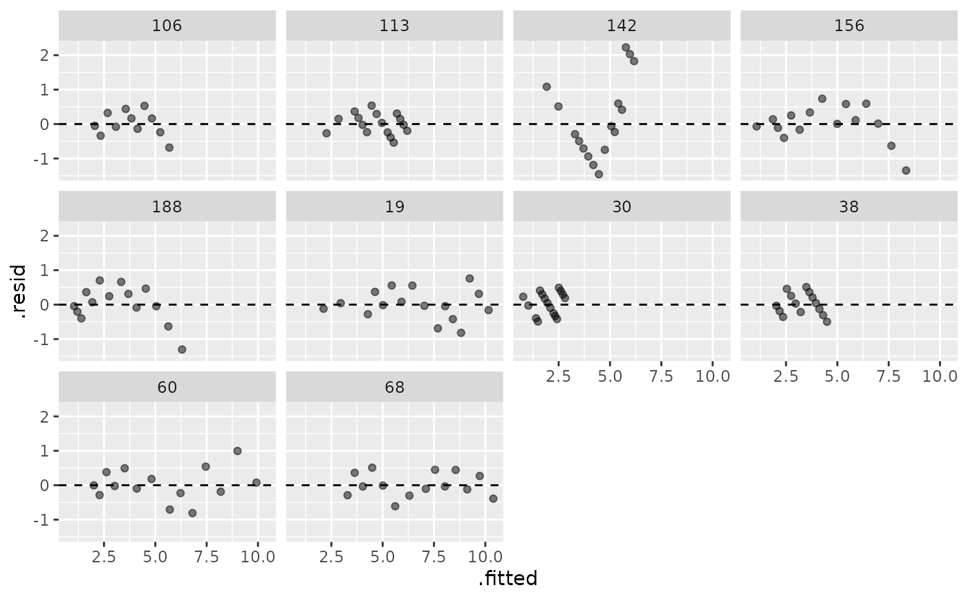
# Plot residuals by subject
library(ggplot2)
ggplot(augmented, aes(x = .fitted, y = .resid)) +
  geom_point(alpha = 0.5) +
  facet_wrap(~id) +
  geom_hline(yintercept = 0, linetype = "dashed")

# }