Augment a beezdemand_hurdle Model with Fitted Values and Residuals
Source:R/hurdle-methods.R
augment.beezdemand_hurdle.RdReturns the original data with fitted values, residuals, and predictions from a hurdle demand model. This enables easy model diagnostics and visualization with the tidyverse.
Usage
# S3 method for class 'beezdemand_hurdle'
augment(x, newdata = NULL, ...)Value
A tibble containing the original data plus:
- .fitted
Fitted demand values (natural scale)
- .fitted_link
Fitted values on log scale (Part II mean)
- .fitted_prob
Predicted probability of consumption (1 - P(zero))
- .resid
Residuals on log scale for positive observations, NA for zeros
- .resid_response
Residuals on response scale (y - .fitted)
Details
For two-part hurdle models:
.fittedgives predicted demand on the natural consumption scale.fitted_probgives the predicted probability of positive consumption.residis defined only for positive observations as log(y) - .fitted_linkObservations with zero consumption have
.resid = NAsince they are explained by Part I (the zero-probability component), not Part II
Examples
# \donttest{
data(apt)
fit <- fit_demand_hurdle(apt, y_var = "y", x_var = "x", id_var = "id")
#> Sample size may be too small for reliable estimation.
#> Subjects: 10, Parameters: 12, Recommended minimum: 60 subjects.
#> Consider using more subjects or the simpler 2-RE model.
#> Fitting HurdleDemand3RE model...
#> Part II: zhao_exponential
#> Subjects: 10, Observations: 160
#> Fixed parameters: 12, Random effects per subject: 3
#> Optimizing...
#> Converged in 81 iterations
#> Computing standard errors...
#> Done. Log-likelihood: 32.81
augmented <- augment(fit)
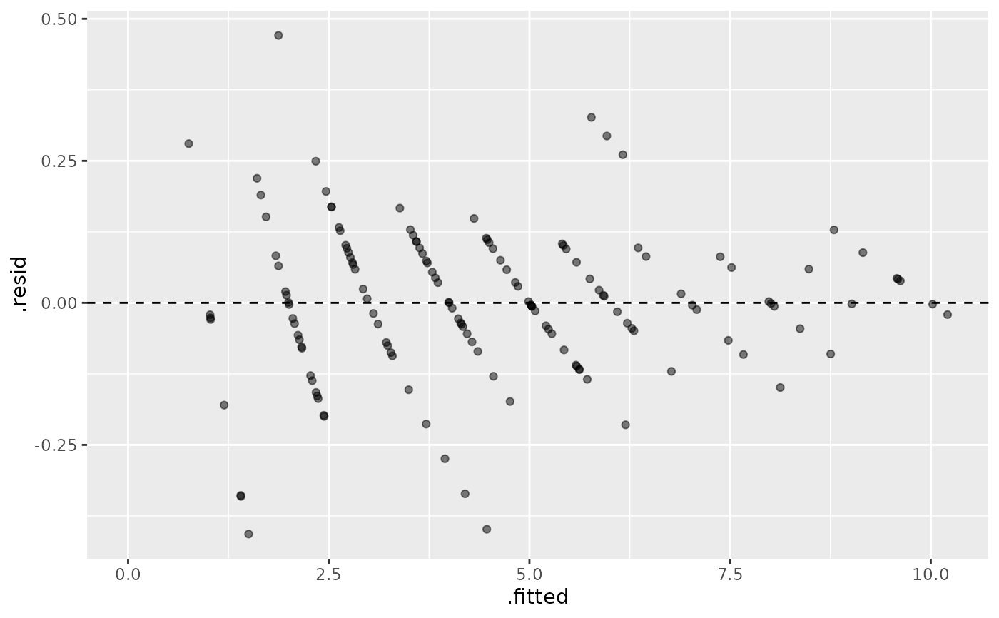
# Plot residuals
library(ggplot2)
ggplot(augmented, aes(x = .fitted, y = .resid)) +
geom_point(alpha = 0.5) +
geom_hline(yintercept = 0, linetype = "dashed")
#> Warning: Removed 14 rows containing missing values or values outside the scale range
#> (`geom_point()`).
 # }
# }