Calculates empirical (model-free) measures of demand from purchase task data. These metrics characterize consumption patterns without fitting a demand curve model.
This is the modern replacement for GetEmpirical(), returning a structured
S3 object with dedicated methods for printing, summarizing, and visualizing.
Arguments
- data
A data frame in long format with columns for subject ID, price, and consumption
- x_var
Character string specifying the column name for price (default: "x")
- y_var
Character string specifying the column name for consumption (default: "y")
- id_var
Character string specifying the column name for subject ID (default: "id")
Value
An S3 object of class beezdemand_empirical containing:
measures - Data frame with one row per subject and columns:
id - Subject identifier
Intensity - Consumption at lowest price (demand intensity)
BP0 - Breakpoint 0: first price where consumption = 0
BP1 - Breakpoint 1: last price with non-zero consumption
Omaxe - Empirical Omax: maximum total expenditure (price × consumption)
Pmaxe - Empirical Pmax: price at which maximum expenditure occurs
call - The matched call
data_summary - List with n_subjects, has_zeros, and complete_cases
Details
Empirical Measures
Intensity - The consumption value at the lowest price point. Reflects unrestricted demand or preferred level of consumption.
BP0 (Breakpoint 0) - The first price at which consumption drops to zero. If consumption never reaches zero, BP0 = NA. Indicates the price threshold where the commodity becomes unaffordable or undesirable.
BP1 (Breakpoint 1) - The highest price at which consumption is still non-zero. If all consumption is zero, BP1 = NA. Represents the upper limit of the commodity's value to the consumer.
Omaxe (Empirical Omax) - The maximum observed expenditure across all prices (max of price × consumption). Represents peak spending on the commodity.
Pmaxe (Empirical Pmax) - The price at which maximum expenditure occurs. If maximum expenditure is zero, Pmaxe = 0. If multiple prices have the same maximum expenditure, the highest price is returned.
Note
Data must not contain duplicate prices within a subject (will error)
Missing values (NA) in consumption are preserved in calculations where applicable
Breakpoints require at least one zero consumption value to be meaningful
See also
GetEmpirical()- Legacy function (superseded)plot.beezdemand_empirical()- Visualization methodsummary.beezdemand_empirical()- Extended summary
Examples
# \donttest{
data(apt, package = "beezdemand")
# Calculate empirical measures
emp <- get_empirical_measures(apt)
print(emp)
#> Empirical Demand Measures
#> =========================
#>
#> Call:
#> get_empirical_measures(data = apt)
#>
#> Data Summary:
#> Subjects: 10
#> Subjects with zero consumption: Yes
#> Complete cases (no NAs): 6
#>
#> Empirical Measures:
#> id Intensity BP0 BP1 Omaxe Pmaxe
#> 19 10 NA 20 45 15
#> 30 3 NA 20 20 20
#> 38 4 15 10 21 7
#> 60 10 15 10 24 8
#> 68 10 15 10 36 9
#> 106 5 8 7 15 5
#> 113 6 NA 20 45 15
#> 142 8 NA 20 60 20
#> 156 7 20 15 21 7
#> 188 5 15 10 15 5
# View measures table
emp$measures
#> id Intensity BP0 BP1 Omaxe Pmaxe
#> 1 19 10 NA 20 45 15
#> 2 30 3 NA 20 20 20
#> 3 38 4 15 10 21 7
#> 4 60 10 15 10 24 8
#> 5 68 10 15 10 36 9
#> 6 106 5 8 7 15 5
#> 7 113 6 NA 20 45 15
#> 8 142 8 NA 20 60 20
#> 9 156 7 20 15 21 7
#> 10 188 5 15 10 15 5
# Extended summary with distribution info
summary(emp)
#> Extended Summary of Empirical Demand Measures
#> =============================================
#>
#> Data Overview:
#> Number of subjects: 10
#> Complete cases: 6 (60.0%)
#>
#> Descriptive Statistics for Empirical Measures:
#> -----------------------------------------------
#>
#> Intensity:
#> Min: 3.00
#> Median: 6.50
#> Mean: 6.80
#> Max: 10.00
#> SD: 2.62
#>
#> BP0:
#> Min: 8.00
#> Median: 15.00
#> Mean: 14.67
#> Max: 20.00
#> SD: 3.83
#> Missing: 4 (40.0%)
#>
#> BP1:
#> Min: 7.00
#> Median: 12.50
#> Mean: 14.20
#> Max: 20.00
#> SD: 5.35
#>
#> Omaxe:
#> Min: 15.00
#> Median: 22.50
#> Mean: 30.20
#> Max: 60.00
#> SD: 15.40
#>
#> Pmaxe:
#> Min: 5.00
#> Median: 8.50
#> Mean: 11.10
#> Max: 20.00
#> SD: 5.88
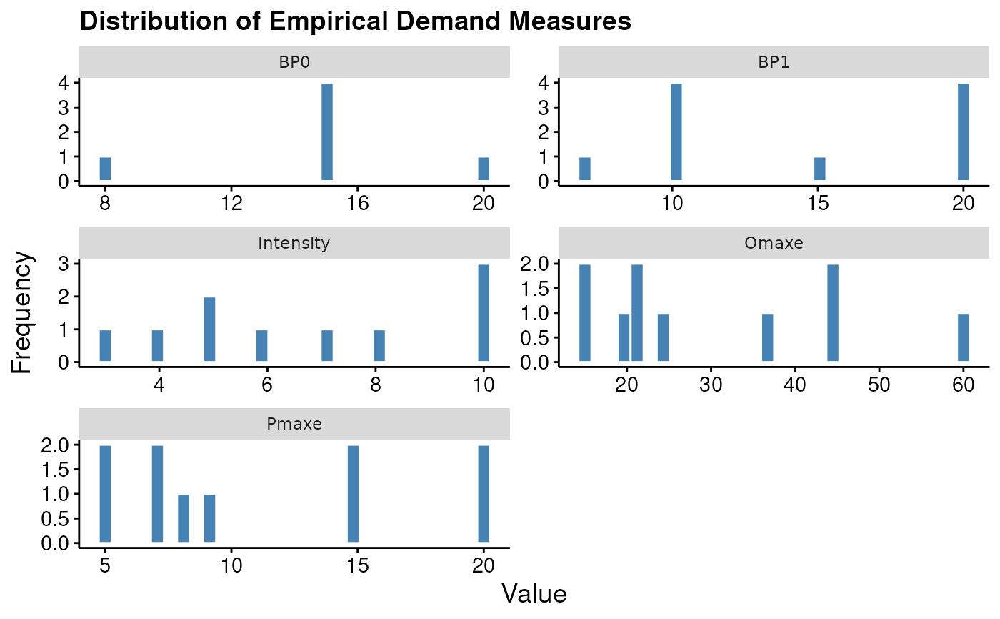
# Visualize distribution of measures
plot(emp) # histogram by default
#> Warning: Removed 4 rows containing non-finite outside the scale range (`stat_bin()`).
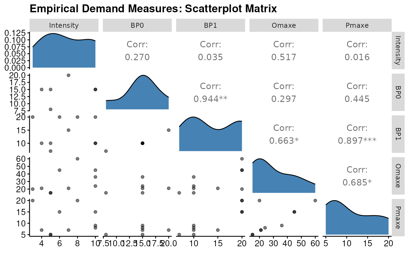
 plot(emp, type = "matrix") # scatterplot matrix
#> Warning: Removed 4 rows containing missing values
#> Warning: Removed 4 rows containing missing values or values outside the scale range
#> (`geom_point()`).
#> Warning: Removed 4 rows containing non-finite outside the scale range
#> (`stat_density()`).
#> Warning: Removed 4 rows containing missing values
#> Warning: Removed 4 rows containing missing values
#> Warning: Removed 4 rows containing missing values
#> Warning: Removed 4 rows containing missing values or values outside the scale range
#> (`geom_point()`).
#> Warning: Removed 4 rows containing missing values or values outside the scale range
#> (`geom_point()`).
#> Warning: Removed 4 rows containing missing values or values outside the scale range
#> (`geom_point()`).
plot(emp, type = "matrix") # scatterplot matrix
#> Warning: Removed 4 rows containing missing values
#> Warning: Removed 4 rows containing missing values or values outside the scale range
#> (`geom_point()`).
#> Warning: Removed 4 rows containing non-finite outside the scale range
#> (`stat_density()`).
#> Warning: Removed 4 rows containing missing values
#> Warning: Removed 4 rows containing missing values
#> Warning: Removed 4 rows containing missing values
#> Warning: Removed 4 rows containing missing values or values outside the scale range
#> (`geom_point()`).
#> Warning: Removed 4 rows containing missing values or values outside the scale range
#> (`geom_point()`).
#> Warning: Removed 4 rows containing missing values or values outside the scale range
#> (`geom_point()`).
 # }
# }