Plot Residual Diagnostics

Creates diagnostic plots for model residuals including residuals vs fitted, scale-location, and histogram of residuals.

Usage

plot_residuals(
  object,
  type = c("all", "fitted", "histogram", "qq"),
  component = c("combined", "continuous"),
  ...
)

Arguments

object

A fitted model object.

type

Character; type of residual plot. One of:

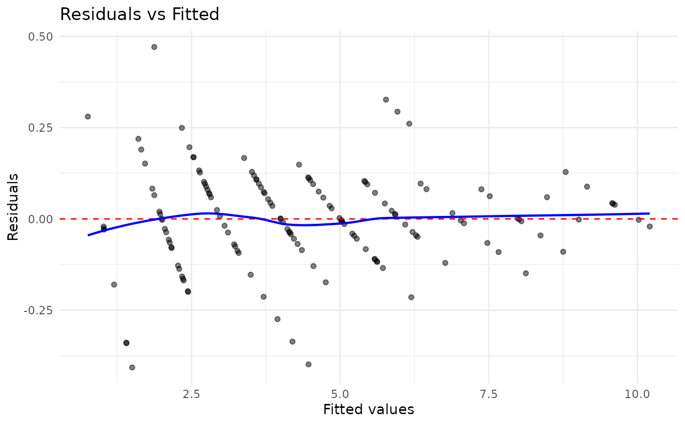
• "fitted": Residuals vs fitted values

• "histogram": Histogram of residuals

• "qq": Q-Q plot of residuals

• "all": All plots combined (default)

component

Character; for hurdle models, which residuals to plot: "combined" (default) uses randomized quantile residuals that assess both binary and continuous components simultaneously; "continuous" uses log-scale Part II residuals only (zeros excluded). Ignored for non-hurdle models.

...

Additional arguments passed to plotting functions.

Value

A ggplot2 object or list of ggplot2 objects.

Details

For hurdle models, diagnostic plots default to randomized quantile residuals that assess both the binary and continuous components simultaneously. Set component = "continuous" to see only Part II (log-scale) residuals.

Examples

# \donttest{
data(apt)
fit <- fit_demand_hurdle(apt, y_var = "y", x_var = "x", id_var = "id")
#> Sample size may be too small for reliable estimation.
#>   Subjects: 10, Parameters: 12, Recommended minimum: 60 subjects.
#>   Consider using more subjects or the simpler 2-RE model.
#> Fitting HurdleDemand3RE model...
#>   Part II: zhao_exponential
#>   Subjects: 10, Observations: 160
#>   Fixed parameters: 12, Random effects per subject: 3
#>   Optimizing...
#>   Converged in 81 iterations
#>   Computing standard errors...
#> Done. Log-likelihood: 32.81
plot_residuals(fit)
#> `geom_smooth()` using formula = 'y ~ x'

# }