S3 Methods for beezdemand_descriptive Objects

Methods for printing, summarizing, and visualizing objects of class beezdemand_descriptive created by get_descriptive_summary().

Usage

# S3 method for class 'beezdemand_descriptive'
print(x, ...)

# S3 method for class 'beezdemand_descriptive'
summary(object, ...)

# S3 method for class 'beezdemand_descriptive'
plot(x, x_trans = "identity", y_trans = "identity", show_zeros = FALSE, ...)

Arguments

x, object: A beezdemand_descriptive object
...: Additional arguments (currently unused)
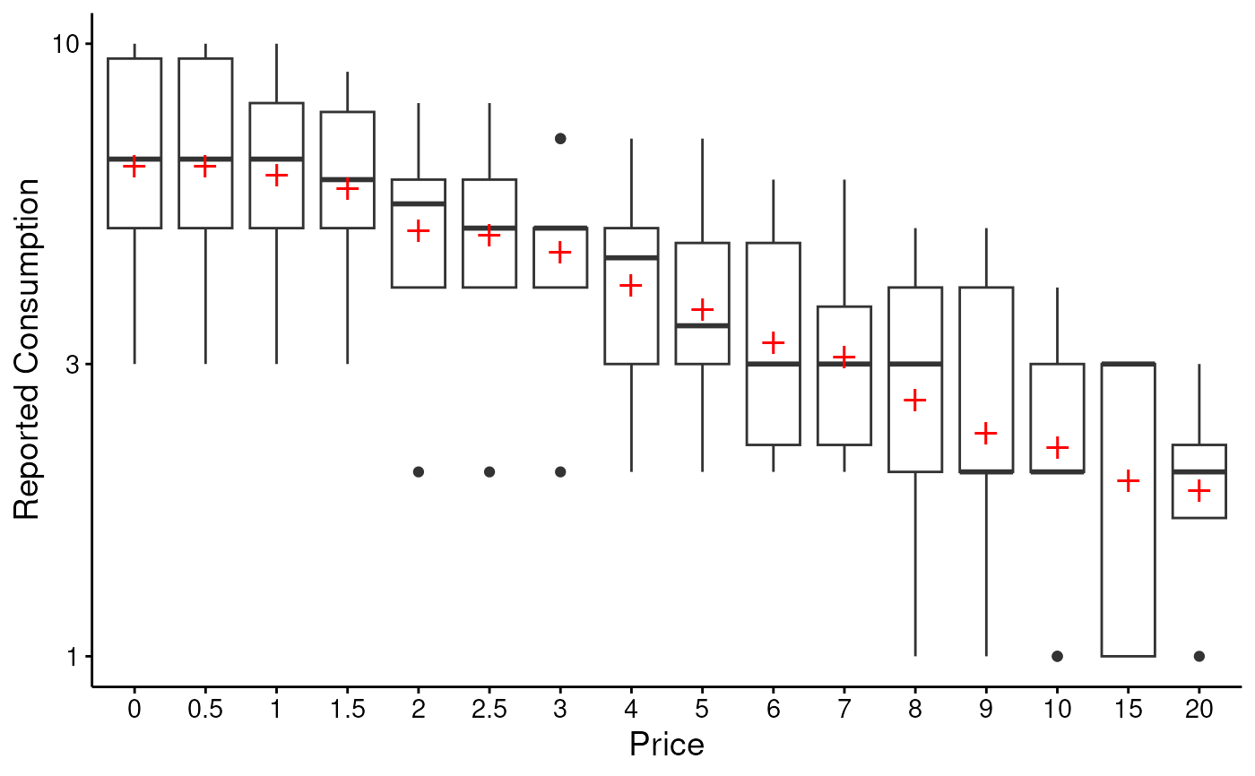
x_trans: Character string specifying x-axis transformation. Options: "identity" (default), "log10", "log", "sqrt". See scales::transform_log10() etc.
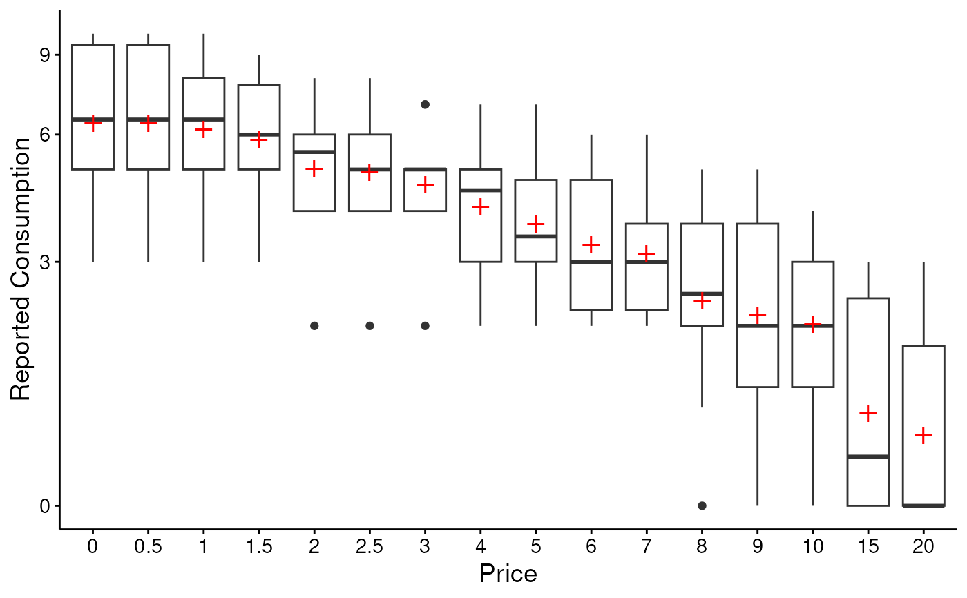
y_trans: Character string specifying y-axis transformation. Options: "identity" (default), "log10", "log", "sqrt", "pseudo_log" (signed log).
show_zeros: Logical indicating whether to show proportion of zeros as labels on the boxplot (default: FALSE)

Value

print() - Returns the object invisibly (called for side effects)
summary() - Returns a list with extended summary information
plot() - Returns a ggplot2 object

Details

Print Method

Displays a compact summary showing the number of subjects and prices analyzed, plus a preview of the statistics table.

Summary Method

Provides extended information including:

Data summary (subjects, prices analyzed)
Distribution of means across prices (min, median, max)
Proportion of zeros by price (range)
Missing data summary

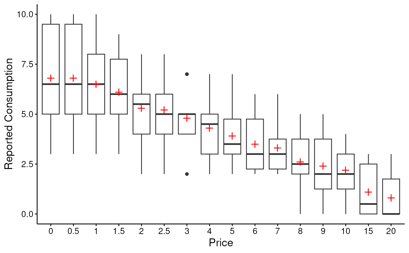
Plot Method

Creates a boxplot showing the distribution of consumption at each price point. Features:

Red cross markers indicate means
Boxes show median and quartiles
Whiskers extend to 1.5 * IQR
Supports axis transformations (log, sqrt, etc.)
Uses modern beezdemand styling via theme_apa()

Examples

# \donttest{
data(apt, package = "beezdemand")
desc <- get_descriptive_summary(apt)

# Print compact summary
print(desc)
#> Descriptive Summary of Demand Data
#> ===================================
#> 
#> Call:
#> get_descriptive_summary(data = apt)
#> 
#> Data Summary:
#>   Subjects: 10
#>   Prices analyzed: 16
#> 
#> Statistics by Price:
#>  Price Mean Median   SD PropZeros NAs Min Max
#>      0  6.8    6.5 2.62       0.0   0   3  10
#>    0.5  6.8    6.5 2.62       0.0   0   3  10
#>      1  6.5    6.5 2.27       0.0   0   3  10
#>    1.5  6.1    6.0 1.91       0.0   0   3   9
#>      2  5.3    5.5 1.89       0.0   0   2   8
#>    2.5  5.2    5.0 1.87       0.0   0   2   8
#>      3  4.8    5.0 1.48       0.0   0   2   7
#>      4  4.3    4.5 1.57       0.0   0   2   7
#>      5  3.9    3.5 1.45       0.0   0   2   7
#>      6  3.5    3.0 1.43       0.0   0   2   6
#>      7  3.3    3.0 1.34       0.0   0   2   6
#>      8  2.6    2.5 1.51       0.1   0   0   5
#>      9  2.4    2.0 1.58       0.1   0   0   5
#>     10  2.2    2.0 1.32       0.1   0   0   4
#>     15  1.1    0.5 1.37       0.5   0   0   3
#>     20  0.8    0.0 1.14       0.6   0   0   3

# Extended summary
summary(desc)
#> Extended Summary of Descriptive Statistics
#> ==========================================
#> 
#> Data Overview:
#>   Number of subjects: 10
#>   Number of prices: 16
#>   Price range: 0 to 9
#> 
#> Distribution of Mean Consumption Across Prices:
#>   Minimum: 0.80
#>   Median: 4.10
#>   Maximum: 6.80
#> 
#> Proportion of Zeros by Price:
#>   Range: 0.00 to 0.60
#> 
#> Missing Data:
#>   No missing values detected

# Default boxplot
plot(desc)


# With log-transformed y-axis
plot(desc, y_trans = "log10")
#> Warning: log-10 transformation introduced infinite values.
#> Warning: log-10 transformation introduced infinite values.
#> Warning: Removed 14 rows containing non-finite outside the scale range
#> (`stat_boxplot()`).
#> Warning: Removed 14 rows containing non-finite outside the scale range
#> (`stat_summary()`).


# With pseudo-log y-axis (handles zeros gracefully)
plot(desc, y_trans = "pseudo_log")

# }