Fit Mixed-Effects Demand Models via TMB

Fits nonlinear mixed-effects demand models using Template Model Builder (TMB) for exact automatic differentiation and Laplace approximation. This provides reliable convergence where traditional NLME approaches fail.

Usage

fit_demand_tmb(
  data,
  y_var = "y",
  x_var = "x",
  id_var = "id",
  equation = c("exponentiated", "exponential", "simplified", "zben"),
  estimate_k = TRUE,
  k = NULL,
  random_effects = Q0 + alpha ~ 1,
  covariance_structure = c("pdSymm", "pdDiag"),
  factors = NULL,
  factor_interaction = FALSE,
  continuous_covariates = NULL,
  collapse_levels = NULL,
  start_values = NULL,
  tmb_control = list(iter_max = 1000, eval_max = 2000),
  multi_start = TRUE,
  validate_subject_pars = TRUE,
  verbose = 1,
  ...,
  store_report_cov = FALSE
)

Arguments

data

A data frame in long format with columns for subject ID, price, and consumption.

y_var

Character. Name of the consumption/response variable.

x_var

Character. Name of the price variable.

id_var

Character. Name of the subject identifier variable.

equation

Character. The demand equation to fit. One of:

"exponentiated": Koffarnus et al. (2015). Gaussian on raw Q. Zeros allowed. Has k parameter.
"exponential": Hursh & Silberberg (2008). Gaussian on log(Q). Observations with Q = 0 are automatically dropped. Has k parameter.
"simplified": Simplified exponential (no k). Gaussian on raw Q. Zeros allowed.
"zben": Zero-bounded exponential (no k). Gaussian on LL4- transformed Q. User must pass LL4-transformed y_var. Note: Q0 on the log10 scale is clamped to a minimum of 0.001 to avoid a singularity at Q0 = 1 (where log10(Q0) = 0 causes division by zero in the decay rate). Subjects with estimated Q0 near 1 may have biased parameter estimates.

estimate_k

Logical. If TRUE (default), estimate k as a free parameter. If FALSE, fix k at the value given in k. Only relevant for "exponentiated" and "exponential" equations.

k

Numeric or NULL. Fixed value of k when estimate_k = FALSE. If NULL and estimate_k = FALSE, k defaults to 2.

random_effects

Specification of subject-level random effects. Accepts any of the following, in order of generality:

formula (default): Q0 + alpha ~ 1 – random intercepts on both parameters (equivalent to the legacy c("q0", "alpha") shortcut). Q0 ~ 1 limits REs to Q0. Formulas with a factor-expanded RHS (e.g., Q0 + alpha ~ condition or Q0 + alpha ~ condition - 1) are supported, giving each subject a random effect per factor level. The within-subject factor must vary within each id; pure between-subject factors belong in factors, not in the RE formula.
continuous within-id covariate (random slope): A numeric RHS term such as Q0 + alpha ~ dose_c gives each subject a random slope on that covariate (dose-response demand). The covariate must vary within id for enough subjects and should be centered (and, for dose ladders, typically log10-transformed); see Details. Pair it with continuous_covariates to also estimate the population (fixed) dose slope.
nlme::pdMat: e.g., nlme::pdDiag(Q0 + alpha ~ 1) or nlme::pdSymm(Q0 + alpha ~ condition). Pre-constructed pdMat objects are accepted and their covariance class is honored (overrides covariance_structure).
list of pdMat / nlme::pdBlocked: Multi-block covariance structures like list(pdSymm(Q0+alpha~1), pdDiag(Q0+alpha~cond-1)) are fully supported.
character vector (deprecated): c("q0", "alpha") or "q0". Soft-deprecated in 0.3.0; emits a lifecycle::deprecate_soft() message. Translated internally to the formula Q0 + alpha ~ 1 or Q0 ~ 1.

covariance_structure

"pdSymm" (default; unstructured) or "pdDiag" (diagonal). Applies only when random_effects is a formula; ignored for pre-constructed pdMat / list / pdBlocked inputs.

factors

Character vector of factor variable names for group comparisons.

factor_interaction

Logical. If TRUE and two factors provided, include their interaction.

continuous_covariates

Character vector of continuous covariate names entered as fixed (population) effects on Q0 and alpha. To also let the per-subject dose-response vary, add the same (centered) covariate as a random slope in random_effects (e.g. Q0 + alpha ~ dose_c); the fixed and random parts are sourced separately and recovering the population dose slope requires both.

collapse_levels

Named list for asymmetric factor collapsing. Structure: list(Q0 = list(factor = list(new = c(old))), alpha = list(...)).

start_values

Named list of starting values. If NULL, data-driven defaults are used.

tmb_control

List of control parameters for the optimizer:

optimizer: Character. "nlminb" (default) or "L-BFGS-B". L-BFGS-B can recover from nlminb convergence failures (code 1 or 8).
iter_max: Maximum iterations (default 1000).
eval_max: Maximum function evaluations (default 2000). Only applies to nlminb; L-BFGS-B has no function evaluation limit.
rel_tol: Relative convergence tolerance (default 1e-10). Only applies to nlminb.
lower: Named numeric vector of lower bounds on optimizer-scale parameters (default NULL = no bounds). Names must match optimizer parameter names (e.g., log_k, beta_q0, logsigma_b). Note that most parameters are in log-space: e.g., to constrain k between 0.14 and 55, use lower = c(log_k = -2), upper = c(log_k = 4). A bound name applies to all occurrences of that parameter (e.g., both elements of beta_q0).
upper: Named numeric vector of upper bounds (see lower).
warm_start: Named numeric vector of starting values in optimizer space (e.g., from a previous fit$opt$par). When provided, multi_start is automatically disabled. This differs from start_values, which operates in parameter space before TMB::MakeADFun(). Length must match the number of free parameters.
trace: Non-negative integer controlling optimizer trace output (default 0). When not explicitly set, inherits from verbose >= 2.

multi_start

Logical. If TRUE (default), try 3 starting value sets and select the best.

validate_subject_pars

Logical. If TRUE (default), validate that every column of the fixed-effect design matrices is constant within each id before computing subject_pars. When a factor or continuous covariate varies within subject, Q0/alpha/Pmax/Omax are set to NA_real_ for affected subjects and a warning names the offending columns. Set to FALSE to force row-order-dependent values (not recommended; prefer a factor-expanded random-effects formula instead).

verbose

Integer. Verbosity level: 0 = silent, 1 = progress, 2 = debug.

...

Additional arguments (currently unused).

store_report_cov

Logical. Advanced storage control. When FALSE (default), the full covariance matrix of all ADREPORT'd quantities ($sdr$cov) is not materialized, shrinking the saved fit substantially (often >80% on large datasets) with no loss of functionality: no method reads it. Standard errors, cov.fixed, variance components, and all inference are identical either way. Set TRUE only if you need the full joint covariance of derived ADREPORT'd quantities.

Value

An object of class beezdemand_tmb containing:

model: List with coefficients, se, variance_components
subject_pars: Data frame of subject-specific Q0, alpha, Pmax, Omax
tmb_obj: TMB objective function object
opt: Optimization result (normalized across optimizers)
sdr: TMB sdreport object. Its $cov (full covariance of all ADREPORT'd quantities) is not materialized – a scalar NA – unless store_report_cov = TRUE.
converged: Logical convergence indicator
loglik: Log-likelihood at convergence
AIC: Akaike Information Criterion
BIC: Bayesian Information Criterion
data: Original data (after any filtering)
param_info: List of model metadata
formula_details: Design matrix and formula information
collapse_info: Collapse levels information (if used)

Details

Traditional NLME approaches using nlme::nlme() universally fail for demand equations because the PNLS algorithm with numerical finite-difference gradients cannot navigate the likelihood surface. TMB succeeds using exact automatic differentiation, Laplace approximation, and joint marginal likelihood optimization.

When estimate_k = TRUE, k is estimated as a free parameter alongside Q0 and alpha. This typically improves model fit substantially. The conventional fixed-k approach (Hursh & Silberberg, 2008) often overestimates k by 3-8x.

Continuous within-subject random slopes (dose-response). A numeric term in the random-effects formula (e.g. Q0 + alpha ~ dose_c) gives each subject a random slope on a continuous within-id covariate, so intensity and elasticity change with the covariate (dose) at a subject-specific rate. The population (fixed) slope is sourced separately from continuous_covariates; recovering it requires both. The covariate must vary within id for enough subjects (a hard error below 2 informative subjects; a warning below 80\ ladders typically a centered log10 dose) so the random intercept is the subject deviation at the reference value and the intercept/slope covariance is interpretable. No silent transform is applied: an uncentered covariate is still fit, but the intercept/slope correlation is reference-dependent and a warning is emitted. Per-subject parameters at a chosen covariate value are available via get_subject_pars(fit, at = c(dose_c = value)) and predict(fit, type = "parameters", at = ...); the per-subject slope deviations appear as q0_<term> / alpha_<term> columns there and in ranef(), and the variance components are labelled by the covariate term in summary() / VarCorr(). See vignette("tmb-advanced-random-effects") for a worked example.

Error model considerations: The exponentiated and simplified equations use a Gaussian error model on raw consumption (Q), which assigns non-zero density to negative values. For data with many near-zero observations, prefer exponential (Gaussian on log Q, zeros dropped) or zben (Gaussian on LL4-transformed Q, zeros handled by the transformation).

Random-effect variance components are reported by summary() on the log10 scale; see ?summary.beezdemand_tmb for the scale convention and its nlme::VarCorr() equivalence.

Examples

# \donttest{
data(apt)

# Exponential (HS) on log(Q)
fit <- fit_demand_tmb(apt, y_var = "y", x_var = "x", id_var = "id",
                      equation = "exponential")
#> Fitting TMB mixed-effects demand model...
#>   Equation: exponential
#>   equation='exponential': Dropped 14 zero-consumption observations (146 remaining).
#>   Subjects: 10, Observations: 146
#>   Random effects: 2 total RE columns per subject (pdSymm(Q0:1, alpha:1))
#>   Design matrices: X_q0 [146 x 1], X_alpha [146 x 1]
#>   Optimizing...
#>   Multi-start: best NLL = -40.65 (start set 3 of 3)
#>   Converged (NLL = -40.65)
#>   Computing standard errors...
#> Done.
summary(fit)
#> 
#> TMB Mixed-Effects Demand Model Summary
#> ================================================== 
#> 
#> Equation: exponential 
#> Backend: TMB_mixed 
#> Convergence: Yes 
#> Subjects: 10  Observations: 146 
#> 
#> --- Fixed Effects ---
#>               term estimate std.error statistic  p.value
#>     Q0:(Intercept)   6.5120    0.8097   15.0689  < 2e-16
#>  alpha:(Intercept)   0.0030    0.0017  -10.3606  < 2e-16
#>              log_k   0.8955    0.4838    1.8509 0.064184
#>           logsigma  -0.9528    0.2292   -4.1564 3.23e-05
#>           logsigma  -0.7798    0.2302   -3.3879 0.000704
#>         logsigma_e  -1.9498    0.0631  -30.9183  < 2e-16
#>            rho_raw  -0.4675    0.3292   -1.4202 0.155547
#> 
#> --- Variance Components ---
#> (Q0/alpha RE SDs on log10 scale; residual SD on likelihood scale)
#>              Component Estimate
#>     sigma_b (Q0 RE SD)   0.1675
#>  sigma_c (alpha RE SD)   0.1991
#>  sigma_e (Residual SD)   0.1423
#> 
#> --- RE Correlations ---
#>                      Component Estimate
#>  rho_bc (Q0-alpha correlation)  -0.4362
#> 
#> --- Fit Statistics ---
#> Log-likelihood: 40.65 
#> AIC: -67.3 
#> BIC: -46.41 
#> 
#> --- Population Demand Metrics ---
#> Pmax: 11.2377  Omax: 23.8941  Method: analytic_lambert_w
#> 
#> --- Individual Parameter Summaries ---
#>   Q0: Min=2.8370  Med=6.2483  Mean=6.9793  Max=10.2274
#>   alpha: Min=0.0016  Med=0.0034  Mean=0.0034  Max=0.0062
#>   Pmax: Min=5.7902  Med=11.6341  Mean=12.1608  Max=21.1473
#>   Omax: Min=11.7465  Med=21.2007  Mean=26.1542  Max=44.1357
#> 
#> Notes:
#>   * 14 zero-consumption observations dropped for equation='exponential'. 
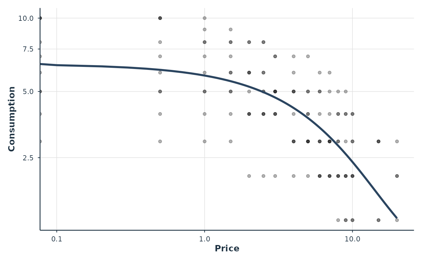
plot(fit)
#> Warning: log-10 transformation introduced infinite values.
#> Warning: log-10 transformation introduced infinite values.


# Exponentiated (Koffarnus) on raw Q
fit2 <- fit_demand_tmb(apt, y_var = "y", x_var = "x", id_var = "id",
                       equation = "exponentiated")
#> Fitting TMB mixed-effects demand model...
#>   Equation: exponentiated
#>   Subjects: 10, Observations: 160
#>   Random effects: 2 total RE columns per subject (pdSymm(Q0:1, alpha:1))
#>   Design matrices: X_q0 [160 x 1], X_alpha [160 x 1]
#>   Optimizing...
#>   Multi-start: best NLL = 171.10 (start set 2 of 3)
#>   WARNING: Did not converge (code 1: false convergence (8))
#>   Computing standard errors...
#> Warning: ! Hessian is not positive definite (`pdHess = FALSE`).
#> ℹ Standard errors, p-values, and confidence intervals may be unreliable.
#> ℹ Run `check_demand_model()` for detailed diagnostics.
#> ℹ Consider simplifying the model (fewer random effects) or checking data
#>   quality.
#> Warning: ! Some standard errors are unavailable (non-positive variance estimates from
#>   `TMB::sdreport()`).
#> ℹ This usually reflects a weakly identified fit; check `$hessian_pd` and
#>   `summary()` diagnostics.
#> Done.

# With covariates (a 30-per-gender subset keeps the example fast)
data(apt_full)
ids <- unique(apt_full[c("id", "gender")])
ids <- ids[ids$gender %in% c("Male", "Female"), ]
keep <- unlist(lapply(split(ids$id, ids$gender), head, 30))
dat <- apt_full[apt_full$id %in% keep, ]
fit3 <- fit_demand_tmb(dat, y_var = "y", x_var = "x", id_var = "id",
                       equation = "exponential", factors = "gender")
#> Fitting TMB mixed-effects demand model...
#>   Equation: exponential
#>   equation='exponential': Dropped 370 zero-consumption observations (650 remaining).
#>   Subjects: 59, Observations: 650
#>   Random effects: 2 total RE columns per subject (pdSymm(Q0:1, alpha:1))
#>   Design matrices: X_q0 [650 x 2], X_alpha [650 x 2]
#>   Optimizing...
#>   Multi-start: best NLL = 175.98 (start set 3 of 3)
#>   Converged (NLL = 175.98)
#>   Computing standard errors...
#> Done.
get_demand_param_emms(fit3, param = "alpha")
#> # A tibble: 2 × 6
#>   level         estimate estimate_log std.error conf.low conf.high
#>   <chr>            <dbl>        <dbl>     <dbl>    <dbl>     <dbl>
#> 1 gender=Female  0.00811        -4.81     0.202  0.00546    0.0121
#> 2 gender=Male    0.00835        -4.79     0.183  0.00583    0.0119
# }

# Factor-expanded random slopes on a within-subject factor are supported
# through the `random_effects` formula interface, e.g.
#   random_effects = nlme::pdDiag(Q0 + alpha ~ cond)
# so each subject contributes a Q0 / alpha random effect per factor level.
# See vignette("tmb-advanced-random-effects", package = "beezdemand").

Usage

Arguments

Value

Details

See also

Examples