TMB Mixed-Effects Demand Models

Introduction

fit_demand_tmb() fits continuous mixed-effects demand models using Template Model Builder (TMB). It is the modern alternative to fit_demand_mixed() (which uses nlme) and provides several advantages:

Automatic differentiation – exact gradients via compiled C++, replacing the numerical finite-difference approximations used by nlme
Laplace approximation – integrates over random effects analytically rather than relying on iterative linearization
Multi-start optimization – automatically tries multiple starting-value sets and keeps the best fit
Four equation forms – exponential, exponentiated, simplified, and zero-bounded exponential (zben)
Factor and covariate support – design matrices for group comparisons with estimated marginal means (EMMs) and pairwise contrasts

This vignette covers fit_demand_tmb() for continuous consumption data. For two-part hurdle models that explicitly model zero consumption, see vignette("hurdle-demand-models"). For individual NLS curves, see vignette("fixed-demand").

Quick Start

fit <- fit_demand_tmb(
  dat,
  y_var = "y", x_var = "x", id_var = "id",
  equation = "exponential",
  random_effects = c("q0", "alpha"),
  verbose = 0
)
fit
#> 
#> TMB Mixed-Effects Demand Model
#> 
#> Call:
#> fit_demand_tmb(data = dat, y_var = "y", x_var = "x", id_var = "id", 
#>     equation = "exponential", random_effects = c("q0", "alpha"), 
#>     verbose = 0)
#> 
#> Equation: exponential 
#> Convergence: Yes 
#> Number of subjects: 99 
#> Number of observations: 1131 
#> Observations dropped (zeros): 569 
#> Random effects: 2 (q0, alpha) 
#> Log-likelihood: -268.54 
#> AIC: 551.07 
#> 
#> Fixed Effects:
#>       Q0.0    alpha.0      log_k   logsigma   logsigma logsigma_e    rho_raw 
#>     1.6944    -4.5060     0.3399    -0.2940    -0.0952    -1.4906    -0.4812 
#> 
#> Use summary() for full results.

summary(fit)
#> 
#> TMB Mixed-Effects Demand Model Summary
#> ================================================== 
#> 
#> Equation: exponential 
#> Backend: TMB_mixed 
#> Convergence: Yes 
#> Subjects: 99  Observations: 1131 
#> 
#> --- Fixed Effects ---
#>               term estimate std.error statistic  p.value
#>     Q0:(Intercept)   5.4434    0.4171   22.1140  < 2e-16
#>  alpha:(Intercept)   0.0110    0.0012  -42.4332  < 2e-16
#>              log_k   0.3399    0.0276   12.2980  < 2e-16
#>           logsigma  -0.2940    0.0748   -3.9297 8.51e-05
#>           logsigma  -0.0952    0.0807   -1.1796 0.238169
#>         logsigma_e  -1.4906    0.0231  -64.4070  < 2e-16
#>            rho_raw  -0.4812    0.1310   -3.6742 0.000239
#> 
#> --- Variance Components ---
#> (Q0/alpha RE SDs on log10 scale; residual SD on likelihood scale)
#>              Component Estimate
#>     sigma_b (Q0 RE SD)   0.3237
#>  sigma_c (alpha RE SD)   0.3948
#>  sigma_e (Residual SD)   0.2252
#> 
#> --- RE Correlations ---
#>                      Component Estimate
#>  rho_bc (Q0-alpha correlation)  -0.4472
#> 
#> --- Fit Statistics ---
#> Log-likelihood: -268.54 
#> AIC: 551.07 
#> BIC: 586.29 
#> 
#> --- Population Demand Metrics ---
#> Pmax: 8.6507  Omax: 12.6853  Method: analytic_lambert_w
#> 
#> --- Individual Parameter Summaries ---
#>   Q0: Min=1.0764  Med=5.8144  Mean=6.9916  Max=27.2637
#>   alpha: Min=0.0012  Med=0.0117  Mean=0.0180  Max=0.1803
#>   Pmax: Min=0.3701  Med=8.9913  Mean=10.5038  Max=54.8223
#>   Omax: Min=0.7770  Med=11.9321  Mean=17.2419  Max=120.2688
#> 
#> Notes:
#>   * 569 zero-consumption observations dropped for equation='exponential'.

plot(fit, type = "demand")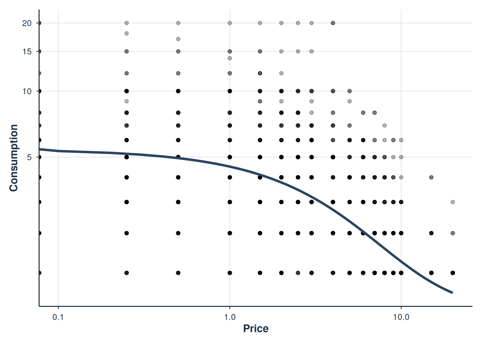

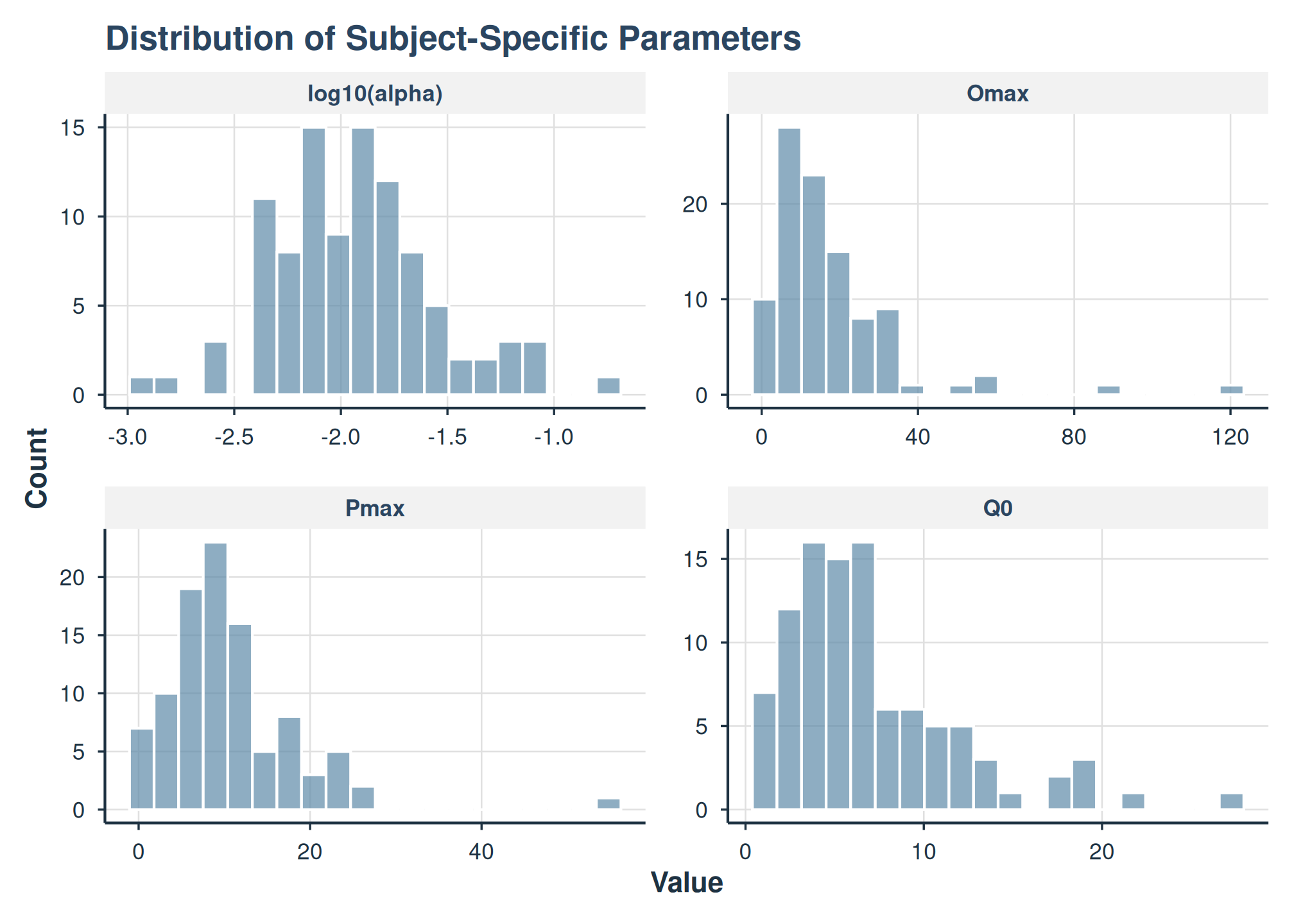
Population demand curve from the exponential equation.

The exponential equation (Hursh & Silberberg, 2008) models log-transformed consumption and is the most reliable choice for 2-random-effect models. It automatically drops zero-consumption observations.

Choosing an Equation

fit_demand_tmb() supports four demand equations:

Equation	Response	Zeros	k	Best for
`"exponential"`	log(Q)	Dropped	Estimated or fixed	Most datasets; robust 2-RE convergence
`"exponentiated"`	Raw Q	Allowed	Estimated or fixed	Data with few zeros; 1-RE models
`"simplified"`	Raw Q	Allowed	None	Simpler model without k
`"zben"`	LL4(Q)	Allowed (via transform)	None	Wide dynamic range with LL4 compression

Mathematical Specifications

Exponential (Hursh & Silberberg, 2008): \log(Q_{ij}) = \log(Q_{0i}) + k \left(e^{-\alpha_i \cdot Q_{0i} \cdot C_j} - 1\right) + \varepsilon_{ij}

Exponentiated (Koffarnus et al., 2015): Q_{ij} = Q_{0i} \cdot 10^{k \left(e^{-\alpha_i \cdot Q_{0i} \cdot C_j} - 1\right)} + \varepsilon_{ij}

Simplified: Q_{ij} = Q_{0i} \cdot e^{-\alpha_i \cdot Q_{0i} \cdot C_j} + \varepsilon_{ij}

Zero-bounded exponential (zben) (see src/MixedDemand.h for full specification): \log_{10}(Q_{0i}) \cdot e^{-\frac{\alpha_i}{\log_{10}(Q_{0i})} \cdot Q_{0i} \cdot C_j} + \varepsilon_{ij}

where Q_{0i} = \exp(\mathbf{x}_i^\top \boldsymbol{\beta}_{Q_0} + b_i), \alpha_i = \exp(\mathbf{x}_i^\top \boldsymbol{\beta}_\alpha + c_i), and (b_i, c_i) are correlated random effects.

fit_exp <- fit_demand_tmb(dat, equation = "exponential",
                          random_effects = c("q0", "alpha"), verbose = 0)

# exponentiated converges reliably with 1-RE
fit_expon <- fit_demand_tmb(dat, equation = "exponentiated",
                            random_effects = "q0", verbose = 0)

fit_simp <- fit_demand_tmb(dat, equation = "simplified",
                           random_effects = "q0", verbose = 0)

dat$y_ll4 <- ll4(dat$y)
fit_zben <- fit_demand_tmb(dat, y_var = "y_ll4", equation = "zben",
                           random_effects = "q0", verbose = 0)

data.frame(
  equation = c("exponential", "exponentiated", "simplified", "zben"),
  random_effects = c("2-RE", "1-RE", "1-RE", "1-RE"),
  converged = c(fit_exp$converged, fit_expon$converged,
                fit_simp$converged, fit_zben$converged),
  AIC = round(c(AIC(fit_exp), AIC(fit_expon),
                AIC(fit_simp), AIC(fit_zben)), 1)
)
#>        equation random_effects converged    AIC
#> 1   exponential           2-RE      TRUE  551.1
#> 2 exponentiated           1-RE      TRUE 6744.5
#> 3    simplified           1-RE      TRUE 6743.4
#> 4          zben           1-RE      TRUE -893.6

Note: AIC values are not directly comparable across equations because they model different response scales (log Q vs raw Q vs LL4(Q)).

Convergence tip: The exponential equation is the most reliable for 2-random-effect models. The exponentiated equation works well with 1-RE but can struggle to converge with 2-RE, especially with smaller samples.

Random Effects Structure

fit_demand_tmb() supports two configurations:

random_effects = "q0" – 1-RE: random intercept on Q_0 only; \alpha is constant across subjects
random_effects = c("q0", "alpha") – 2-RE: random effects on both Q_0 and \alpha with an estimated correlation

fit_1re <- fit_demand_tmb(dat, equation = "exponential",
                          random_effects = "q0", verbose = 0)
fit_2re <- fit  # reuse from Quick Start (exponential, 2-RE)

compare_models(fit_1re, fit_2re)
#> 
#> Model Comparison
#> ================================================== 
#> 
#>    Model          Class   Backend nobs df    logLik       AIC       BIC
#>  Model_1 beezdemand_tmb TMB_mixed 1131  5 -639.5903 1289.1807 1314.3350
#>  Model_2 beezdemand_tmb TMB_mixed 1131  7 -268.5364  551.0729  586.2889
#>  delta_AIC delta_BIC
#>   738.1078  728.0461
#>     0.0000    0.0000
#> 
#> Best model by BIC: Model_2 
#> 
#> Likelihood Ratio Tests:
#> ---------------------------------------- 
#>          Comparison  LR_stat df p_value
#>  Model_1 vs Model_2 742.1078  2  <2e-16
#> 
#> Notes:
#>   - LRT nesting assumption not verified.

A significant LRT p-value and substantially lower AIC/BIC for the 2-RE model indicate that subjects differ meaningfully in both intensity (Q_0) and elasticity (\alpha).

head(nlme::ranef(fit_2re))
#>   id        b_i         c_i q0_(Intercept) alpha_(Intercept)
#> 1 16 -0.8553425  0.38606925     -0.8553425        0.38606925
#> 2 24  0.0892061 -0.04866633      0.0892061       -0.04866633
#> 3 33  0.6114842 -0.35230990      0.6114842       -0.35230990
#> 4 40  0.1527007  0.50021504      0.1527007        0.50021504
#> 5 42  0.7378500 -0.89299758      0.7378500       -0.89299758
#> 6 49 -0.2956502  0.40088468     -0.2956502        0.40088468

The b_i column is the random deviation on log(Q_0) and c_i is the random deviation on log(\alpha) for each subject.

Estimating vs. Fixing k

For the exponential and exponentiated equations, k scales the range of the demand curve. By default it is estimated (estimate_k = TRUE). You can fix it at the conventional value of 2 (Hursh & Silberberg, 2008):

fit_k_free <- fit_demand_tmb(dat, equation = "exponential",
                              random_effects = c("q0", "alpha"),
                              estimate_k = TRUE, verbose = 0)
fit_k_fixed <- fit_demand_tmb(dat, equation = "exponential",
                               random_effects = c("q0", "alpha"),
                               estimate_k = FALSE, k = 2, verbose = 0)

data.frame(
  k = c("estimated", "fixed at 2"),
  converged = c(fit_k_free$converged, fit_k_fixed$converged),
  AIC = round(c(AIC(fit_k_free), AIC(fit_k_fixed)), 1),
  k_value = round(c(exp(coef(fit_k_free)[["log_k"]]), 2), 3)
)
#>            k converged   AIC k_value
#> 1  estimated      TRUE 551.1   1.405
#> 2 fixed at 2      TRUE 607.1   2.000

The simplified and zben equations do not use a k parameter.

Examining Results

Summary and Coefficients

summary(fit_2re)
#> 
#> TMB Mixed-Effects Demand Model Summary
#> ================================================== 
#> 
#> Equation: exponential 
#> Backend: TMB_mixed 
#> Convergence: Yes 
#> Subjects: 99  Observations: 1131 
#> 
#> --- Fixed Effects ---
#>               term estimate std.error statistic  p.value
#>     Q0:(Intercept)   5.4434    0.4171   22.1140  < 2e-16
#>  alpha:(Intercept)   0.0110    0.0012  -42.4332  < 2e-16
#>              log_k   0.3399    0.0276   12.2980  < 2e-16
#>           logsigma  -0.2940    0.0748   -3.9297 8.51e-05
#>           logsigma  -0.0952    0.0807   -1.1796 0.238169
#>         logsigma_e  -1.4906    0.0231  -64.4070  < 2e-16
#>            rho_raw  -0.4812    0.1310   -3.6742 0.000239
#> 
#> --- Variance Components ---
#> (Q0/alpha RE SDs on log10 scale; residual SD on likelihood scale)
#>              Component Estimate
#>     sigma_b (Q0 RE SD)   0.3237
#>  sigma_c (alpha RE SD)   0.3948
#>  sigma_e (Residual SD)   0.2252
#> 
#> --- RE Correlations ---
#>                      Component Estimate
#>  rho_bc (Q0-alpha correlation)  -0.4472
#> 
#> --- Fit Statistics ---
#> Log-likelihood: -268.54 
#> AIC: 551.07 
#> BIC: 586.29 
#> 
#> --- Population Demand Metrics ---
#> Pmax: 8.6507  Omax: 12.6853  Method: analytic_lambert_w
#> 
#> --- Individual Parameter Summaries ---
#>   Q0: Min=1.0764  Med=5.8144  Mean=6.9916  Max=27.2637
#>   alpha: Min=0.0012  Med=0.0117  Mean=0.0180  Max=0.1803
#>   Pmax: Min=0.3701  Med=8.9913  Mean=10.5038  Max=54.8223
#>   Omax: Min=0.7770  Med=11.9321  Mean=17.2419  Max=120.2688
#> 
#> Notes:
#>   * 569 zero-consumption observations dropped for equation='exponential'.

The fixed-effect coefficient table reports estimate and std.error on the scale set by report_space: the default, "natural", back-transforms Q_0, \alpha, and k off the log estimation scale. The statistic and p.value columns are always computed on the estimation (log) scale, where the Wald test is well defined; they are not recomputed from the back-transformed estimate and std.error (that recompute is degenerate for a strictly positive parameter – it would test “ratio = 0” rather than “ratio = 1”). One consequence: estimate / std.error from the default table does not reproduce the reported statistic. This matches the broom and emmeans convention; pass report_space = "internal" (or "log10") to read the estimate and SE on the same scale as the test.

The variance_components block reports the Q_0 and \alpha random-effect standard deviations on the log10 scale. TMB estimates these SDs on the natural-log scale internally; summary() divides them by \log(10) so they are directly comparable with nlme::VarCorr() on a fit_demand_mixed() fit using the default param_space = "log10". The residual SD is reported on the model’s likelihood scale, which is equation-dependent (log-consumption for exponential, the LL4-transformed y_var for zben); the random-effect correlations are scale-invariant.

For users coming from nlme or lme4, the VarCorr() accessor returns these same variance components in the familiar nlme::VarCorr() matrix layout – a Variance / StdDev matrix (with a Corr column for pdSymm fits) and a final Residual row:

VarCorr(fit_2re)
#>          Variance StdDev Corr  
#> Q0       0.1050   0.324        
#> alpha    0.1560   0.395  -0.447
#> Residual 0.0507   0.225

Note that tidy() (shown next) reports the raw internal optimizer parameters instead – the logsigma rows are the natural log of each RE SD, not the log10-scale SDs from summary()$variance_components.

tidy(fit_2re)
#> # A tibble: 6 × 9
#>   term          estimate std.error statistic    p.value component estimate_scale
#>   <chr>            <dbl>     <dbl>     <dbl>      <dbl> <chr>     <chr>         
#> 1 Q0:(Intercep…   5.44     0.417        22.1  2.32e-108 fixed     natural       
#> 2 alpha:(Inter…   0.0110   0.00117     -42.4  0         fixed     natural       
#> 3 log_k           0.340    0.0276       12.3  9.28e- 35 fixed     log           
#> 4 sigma_b (Q0 …   0.324   NA            NA   NA         variance  log10         
#> 5 sigma_c (alp…   0.395   NA            NA   NA         variance  log10         
#> 6 sigma_e (Res…   0.225   NA            NA   NA         variance  natural       
#> # ℹ 2 more variables: term_display <chr>, estimate_internal <dbl>

glance(fit_2re)
#> # A tibble: 1 × 10
#>   model_class  backend equation_form  nobs n_subjects n_random_effects converged
#>   <chr>        <chr>   <chr>         <int>      <int>            <int> <lgl>    
#> 1 beezdemand_… TMB_mi… exponential    1131         99                2 TRUE     
#> # ℹ 3 more variables: logLik <dbl>, AIC <dbl>, BIC <dbl>

Subject-Specific Parameters

Each subject gets empirical Bayes estimates of Q_0, \alpha, P_{max}, and O_{max}:

spars <- get_subject_pars(fit_2re)
head(spars)
#>   id        b_i         c_i        Q0       alpha      Pmax      Omax
#> 1 16 -0.8553425  0.38606925  2.314197 0.016246302 13.830982  8.622529
#> 2 24  0.0892061 -0.04866633  5.951310 0.010518438  8.306997 13.317967
#> 3 33  0.6114842 -0.35230990 10.033098 0.007763911  6.675631 18.042997
#> 4 40  0.1527007  0.50021504  6.341441 0.018210732  4.502903  7.692399
#> 5 42  0.7378500 -0.89299758 11.384528 0.004521295 10.102527 30.983205
#> 6 49 -0.2956502  0.40088468  4.050155 0.016488790  7.786593  8.495724
#>   pmax_at_bound
#> 1         FALSE
#> 2         FALSE
#> 3         FALSE
#> 4         FALSE
#> 5         FALSE
#> 6         FALSE

spars |>
  summarise(
    across(c(Q0, alpha, Pmax, Omax),
           list(median = median, mean = mean, sd = sd),
           .names = "{.col}_{.fn}")
  ) |>
  tidyr::pivot_longer(everything(), names_to = c("parameter", "stat"),
                      names_sep = "_") |>
  tidyr::pivot_wider(names_from = stat, values_from = value) |>
  mutate(across(where(is.numeric), \(x) round(x, 4)))
#> # A tibble: 4 × 4
#>   parameter  median   mean      sd
#>   <chr>       <dbl>  <dbl>   <dbl>
#> 1 Q0         5.81    6.99   5.01  
#> 2 alpha      0.0117  0.018  0.0238
#> 3 Pmax       8.99   10.5    7.53  
#> 4 Omax      11.9    17.2   17.3

Amplitude–Persistence Decomposition

calculate_amplitude_persistence() collapses the per-subject parameters into two latent factors used in behavioral economic indices: Amplitude (intensity of demand, primarily Q_0) and Persistence (sensitivity to price, drawn from P_{max}, O_{max}, and 1/\alpha). The TMB method extracts subject parameters from fit$subject_pars and delegates to the default Z-score implementation, so the result is comparable across model tiers.

ap <- calculate_amplitude_persistence(fit_2re)
head(ap)
#>   id       z_Q0      z_Pmax      z_Omax z_inv_alpha  Amplitude Persistence
#> 1 16 -0.9332306  0.44158011 -0.49884140 -0.49884140 -0.9332306  -0.1853676
#> 2 24 -0.2075582 -0.29156364 -0.22709436 -0.22709436 -0.2075582  -0.2485841
#> 3 33  0.6068353 -0.50807870  0.04636527  0.04636527  0.6068353  -0.1384494
#> 4 40 -0.1297198 -0.79644335 -0.55267242 -0.55267242 -0.1297198  -0.6339294
#> 5 42  0.8764710 -0.05326084  0.79527589  0.79527589  0.8764710   0.5124303
#> 6 49 -0.5868744 -0.36063167 -0.50618019 -0.50618019 -0.5868744  -0.4576640

ap |>
  summarise(
    Amplitude_mean = mean(Amplitude, na.rm = TRUE),
    Persistence_mean = mean(Persistence, na.rm = TRUE),
    Amplitude_sd = sd(Amplitude, na.rm = TRUE),
    Persistence_sd = sd(Persistence, na.rm = TRUE)
  )
#>   Amplitude_mean Persistence_mean Amplitude_sd Persistence_sd
#> 1   7.065932e-18    -2.846441e-18            1      0.8497968

By construction, both factors are sample-standardized (mean 0, SD 1 within the fitted dataset). For cross-sample comparisons, supply external basis_means and basis_sds so the standardization uses a fixed reference.

Confidence Intervals

confint(fit_2re)
#> # A tibble: 7 × 5
#>   term              estimate conf.low conf.high level
#>   <chr>                <dbl>    <dbl>     <dbl> <dbl>
#> 1 Q0:(Intercept)      1.69      1.54     1.84    0.95
#> 2 alpha:(Intercept)  -4.51     -4.71    -4.30    0.95
#> 3 log_k               0.340     0.286    0.394   0.95
#> 4 logsigma           -0.294    -0.441   -0.147   0.95
#> 5 logsigma           -0.0952   -0.254    0.0630  0.95
#> 6 logsigma_e         -1.49     -1.54    -1.45    0.95
#> 7 rho_raw            -0.481    -0.738   -0.225   0.95

By default, confidence intervals are on the internal (log) scale. Use report_space = "natural" for back-transformed intervals:

confint(fit_2re, report_space = "natural")
#> # A tibble: 7 × 5
#>   term              estimate conf.low conf.high level
#>   <chr>                <dbl>    <dbl>     <dbl> <dbl>
#> 1 Q0:(Intercept)      5.44    4.68       6.33    0.95
#> 2 alpha:(Intercept)   0.0110  0.00897    0.0136  0.95
#> 3 log_k               1.40    1.33       1.48    0.95
#> 4 logsigma           -0.294  -0.441     -0.147   0.95
#> 5 logsigma           -0.0952 -0.254      0.0630  0.95
#> 6 logsigma_e         -1.49   -1.54      -1.45    0.95
#> 7 rho_raw            -0.481  -0.738     -0.225   0.95

For a quick diagnostic on the Gaussian (Wald) approximation, request Monte Carlo intervals with method = "simulate". These draw R samples from the joint asymptotic posterior N(coef, vcov) and report empirical quantiles. They are asymptotically Wald-equivalent, so a large discrepancy between the two flags a fit where the Gaussian approximation is suspect. This is a diagnostic comparison, not an accuracy improvement: the simulate method does not capture non-Gaussian posterior shape and carries no positivity guarantee on the internal scale. Set seed for reproducibility.

ci_wald <- confint(fit_2re)
ci_sim <- confint(fit_2re, method = "simulate", R = 2000, seed = 42)
data.frame(
  term = ci_wald$term,
  width_wald = ci_wald$conf.high - ci_wald$conf.low,
  width_sim = ci_sim$conf.high - ci_sim$conf.low
)
#>                term width_wald  width_sim
#> 1    Q0:(Intercept) 0.30035058 0.29461890
#> 2 alpha:(Intercept) 0.41625530 0.42113249
#> 3             log_k 0.10833786 0.10835459
#> 4          logsigma 0.29327780 0.29006254
#> 5          logsigma 0.31651456 0.31452214
#> 6        logsigma_e 0.09071999 0.09080796
#> 7           rho_raw 0.51338445 0.52553410

Variance-Covariance and the Delta Method

vcov() returns the fixed-effect variance-covariance matrix from the TMB sdreport — the inverse of the negative Hessian at the MLE, restricted to fixed effects after Laplace-marginalizing the random effects. Combined with the optimizer’s internal parameter vector (coef(fit, type = "internal")), it lets you apply the delta method to any nonlinear function of the parameters via car::deltaMethod. Pass the parameter vector explicitly so the call is stable across the planned coef() default change in a future release.

beta <- coef(fit_2re, type = "internal")
car::deltaMethod(
  beta,
  paste0(names(beta)[1], " * 1"),
  vcov. = vcov(fit_2re)
)
#>             Estimate       SE    2.5 % 97.5 %
#> beta_q0 * 1 1.694405 0.076621 1.544230 1.8446

fitted(fit) and residuals(fit) are also exposed as direct accessors, matching the model-scale convention used by broom::augment() (log scale for "exponential", natural/LL4 scale for others). Pass scale = "natural" to back-transform.

Predictions

Three prediction types are available:

# Fitted values for observed data
pred_resp <- predict(fit_2re, type = "response")
head(pred_resp)
#> # A tibble: 6 × 9
#>   id    gender   age binges totdrinks tothours     x     y .fitted
#>   <fct> <chr>  <dbl>  <dbl>     <dbl>    <dbl> <dbl> <dbl>   <dbl>
#> 1 16    Male      30      0         1        1  0        2   0.839
#> 2 16    Male      30      0         1        1  0.25     2   0.809
#> 3 16    Male      30      0         1        1  0.5      2   0.779
#> 4 16    Male      30      0         1        1  1        2   0.720
#> 5 16    Male      30      0         1        1  1.5      2   0.662
#> 6 16    Male      30      0         1        1  2        2   0.605

# Population demand curve at specific prices
predict(fit_2re, type = "demand", prices = c(0, 0.5, 1, 2, 5, 10, 20))
#> # A tibble: 7 × 2
#>   price .fitted
#>   <dbl>   <dbl>
#> 1   0     1.69 
#> 2   0.5   1.60 
#> 3   1     1.51 
#> 4   2     1.33 
#> 5   5     0.855
#> 6  10     0.233
#> 7  20    -0.568

# Subject-level parameter estimates (same as get_subject_pars)
pred_pars <- predict(fit_2re, type = "parameters")
head(pred_pars)
#> # A tibble: 6 × 8
#>   id        b_i     c_i    Q0   alpha  Pmax  Omax pmax_at_bound
#>   <chr>   <dbl>   <dbl> <dbl>   <dbl> <dbl> <dbl> <lgl>        
#> 1 16    -0.855   0.386   2.31 0.0162  13.8   8.62 FALSE        
#> 2 24     0.0892 -0.0487  5.95 0.0105   8.31 13.3  FALSE        
#> 3 33     0.611  -0.352  10.0  0.00776  6.68 18.0  FALSE        
#> 4 40     0.153   0.500   6.34 0.0182   4.50  7.69 FALSE        
#> 5 42     0.738  -0.893  11.4  0.00452 10.1  31.0  FALSE        
#> 6 49    -0.296   0.401   4.05 0.0165   7.79  8.50 FALSE

For type = "response", the level argument controls whether predictions condition on subject random effects. level = "subject" (the default) conditions on each subject’s random effects and needs an id column in newdata; level = "population" sets the random effects to zero and needs no id. Requesting both at once returns predict.fixed (population) and predict.id (subject) side by side, matching the nlme::predict.lme(level = 0:1) layout so nlme-based plotting code runs unchanged.

px <- exp(seq(log(0.05), log(20), length.out = 60))
ids_show <- unique(dat$id)[1:6]

pred_levels <- predict(
  fit_2re,
  newdata = expand.grid(x = px, id = ids_show),
  level = c("population", "subject"),
  scale = "natural"
)
head(pred_levels)
#> # A tibble: 6 × 4
#>        x id    predict.fixed predict.id
#>    <dbl> <fct>         <dbl>      <dbl>
#> 1 0.05   16             5.53       2.36
#> 2 0.0553 16             5.52       2.36
#> 3 0.0613 16             5.52       2.36
#> 4 0.0678 16             5.51       2.35
#> 5 0.0751 16             5.50       2.35
#> 6 0.0831 16             5.49       2.35

The population-mean curve is identical for every subject, so a single predict.fixed column overlays the per-subject predict.id curves.

ggplot(pred_levels, aes(x = x)) +
  geom_line(aes(y = predict.id, group = id), colour = "grey65") +
  geom_line(
    data = subset(pred_levels, id == ids_show[1]),
    aes(y = predict.fixed), colour = "#2c3e50", linewidth = 1.2
  ) +
  scale_x_log10() +
  labs(x = "Price", y = "Predicted consumption") +
  theme_minimal()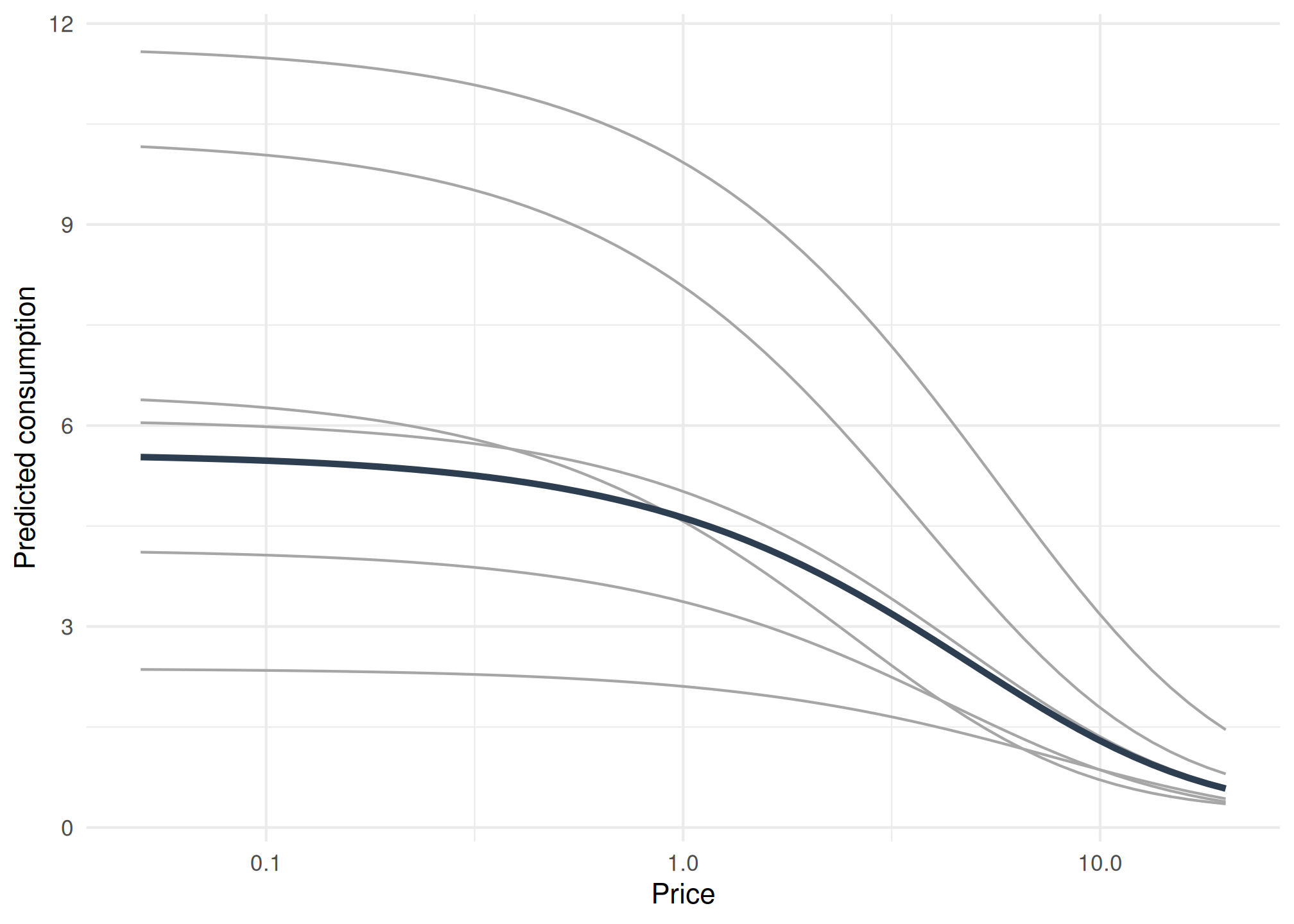

Subject-conditional demand curves (grey) around the population-mean curve (dark).

Population Metrics

calc_group_metrics(fit_2re)
#> $Pmax
#> [1] 8.65068
#> 
#> $Omax
#> [1] 12.68535
#> 
#> $Qmax
#> [1] 1.466399
#> 
#> $elasticity_at_pmax
#> [1] -1
#> 
#> $method
#> [1] "analytic_lambert_w"
#> 
#> $pmax_at_bound
#> [1] FALSE
#> 
#> $conditioned_on
#> NULL

Visualization

plot(fit_2re, type = "demand")

Population-level demand curve with confidence band.

plot(fit_2re, type = "individual")

Individual demand curves for a random sample of subjects.

plot(fit_2re, type = "parameters")

Distribution of subject-specific demand parameters.

Diagnostics

After fitting, assess model health with the built-in diagnostic tools.

The fit object exposes a hessian_pd field that flags whether the Hessian returned by TMB::sdreport() is positive definite. When FALSE, standard errors, p-values, and Wald confidence intervals derived from the Hessian should be treated as unreliable; the warning is also surfaced as a note in summary() output and as a hessian_warning attribute on tidy() output.

fit_2re$hessian_pd
#> [1] TRUE

# Model health check — convergence, variance components, residual stats,
# and (since 0.3.0) Hessian positive-definiteness.
check_demand_model(fit_2re)
#> 
#> Model Diagnostics
#> ================================================== 
#> Model class: beezdemand_tmb 
#> 
#> Convergence:
#>   Status: Converged
#> 
#> Random Effects:
#>   sigma_b variance: 0.3237
#>   sigma_c variance: 0.3948
#> 
#> Residuals:
#>   Mean: -0.0001171
#>   SD: 0.2069
#>   Range: [-0.9401, 0.7515]
#>   Outliers: 12 observations
#> 
#> --------------------------------------------------
#> Issues Detected (1):
#>   1. Detected 12 potential outliers (|resid| > 3 SD)
#> 
#> Recommendations:
#>   - Investigate outlying observations

# Augment with fitted values and residuals
aug <- augment(fit_2re)
head(aug[, c("id", "x", "y", ".fitted", ".resid", ".std_resid")])
#> # A tibble: 6 × 6
#>   id        x     y .fitted  .resid .std_resid
#>   <fct> <dbl> <dbl>   <dbl>   <dbl>      <dbl>
#> 1 16     0        2   0.839 -0.146      -0.648
#> 2 16     0.25     2   0.809 -0.116      -0.513
#> 3 16     0.5      2   0.779 -0.0857     -0.380
#> 4 16     1        2   0.720 -0.0266     -0.118
#> 5 16     1.5      2   0.662  0.0315      0.140
#> 6 16     2        2   0.605  0.0884      0.392

# Q-Q plot of random effects
plot_qq(fit_2re)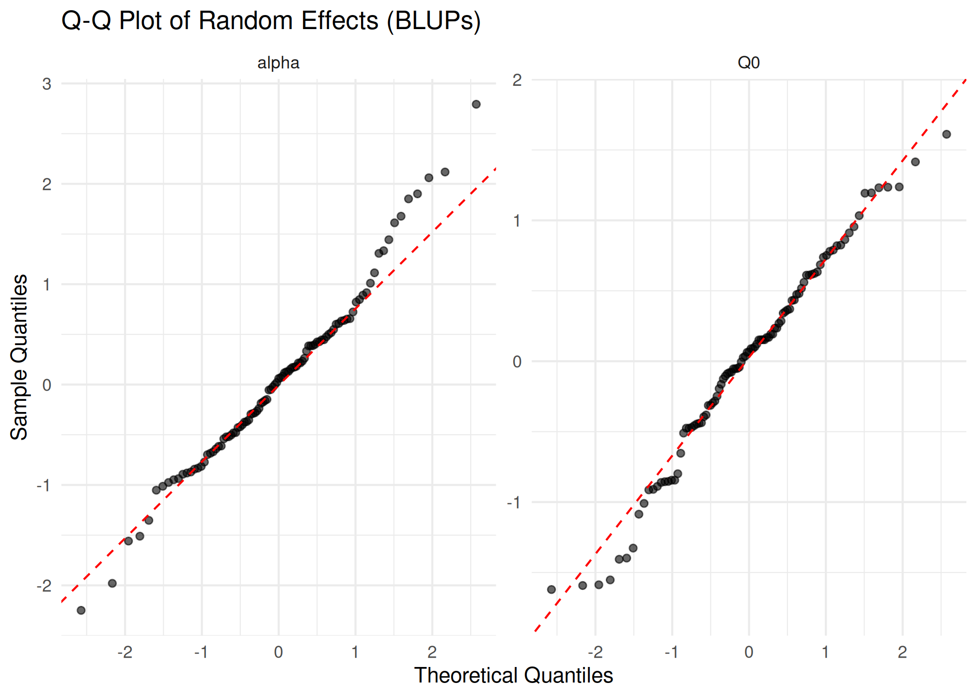

Q-Q plots of subject-level random effects.

# Random effects diagnostic panels
plot_re_diagnostics(fit_2re)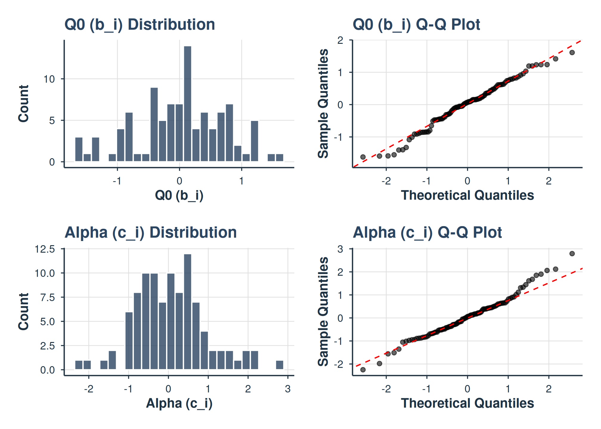

Random effects diagnostic panels.

# Residual plot — standard in every modeling workflow
plot_residuals(fit_2re, type = "fitted")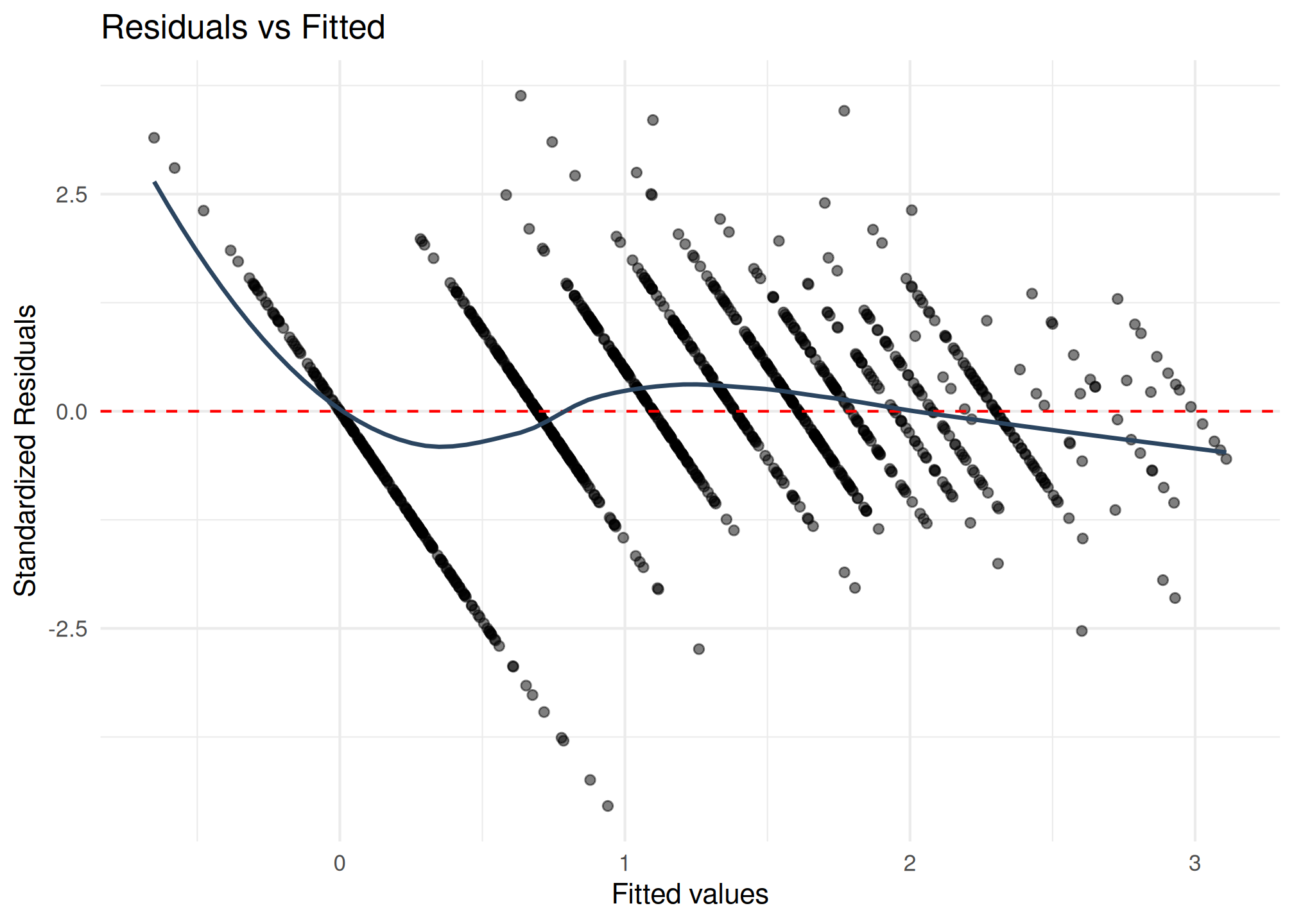

Residuals vs fitted values for the 2-RE exponential model.

These diagnostics help identify:

Q-Q plots: Non-normality of random effects (heavy tails, outliers)
check_demand_model(): Convergence issues, boundary estimates, residual patterns
Augmented data: Observation-level residuals for identifying poorly fitting subjects
Residual plots: Heteroscedasticity, non-linearity, or outliers in the fitted vs residual pattern

Advanced Visualization

beezdemand provides several specialized plots beyond the standard plot() method. These work with any beezdemand_tmb object.

Expenditure and Elasticity

The expenditure curve shows total spending (P \times Q) as a function of price, with vertical and horizontal reference lines at P_{max} and O_{max}:

plot_expenditure(fit_2re)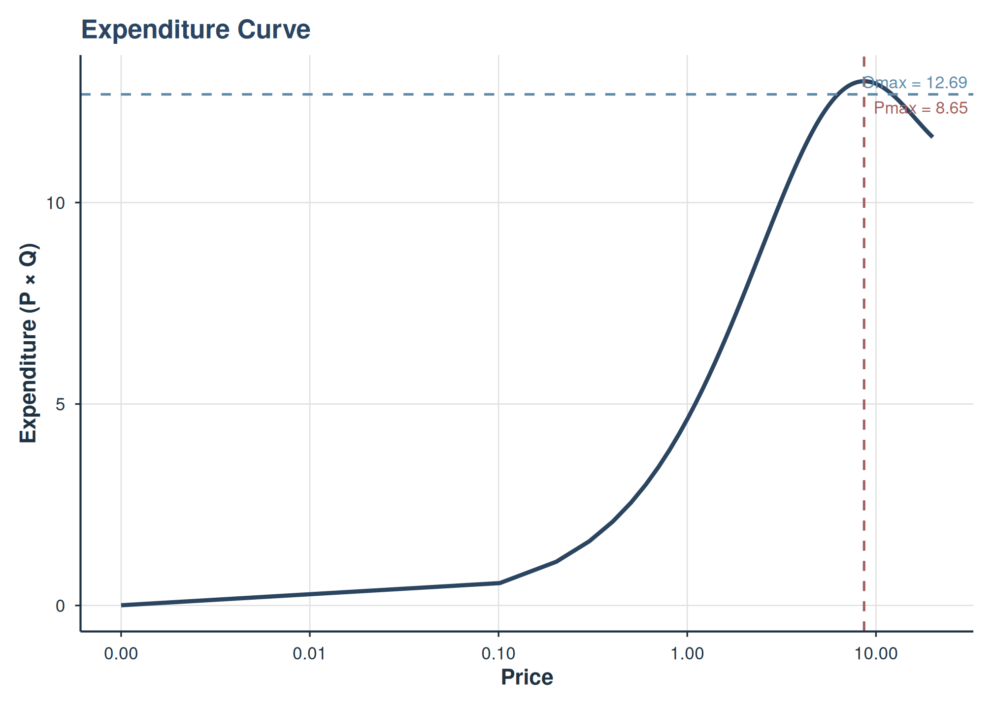

Expenditure curve with Pmax and Omax reference lines.

The elasticity curve shows how responsive demand is to price changes. The dashed line at -1 marks unit elasticity — prices above this threshold produce elastic demand:

plot_elasticity(fit_2re)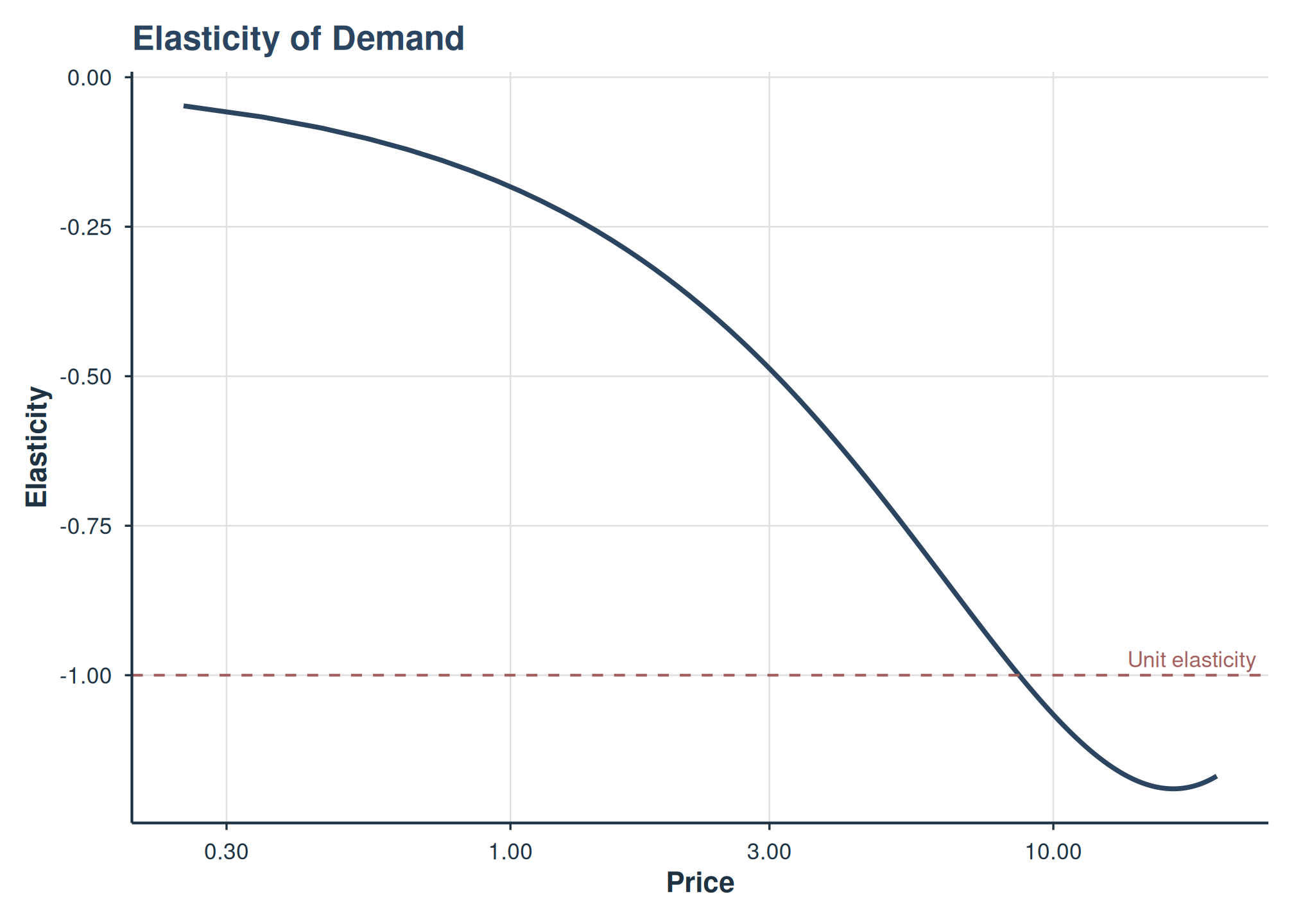

Own-price elasticity curve with unit elasticity reference.

Loss Surface and Profile

The loss surface visualizes the sum-of-squared-residuals landscape over a grid of (Q_0, \alpha) values, with the MLE marked. This helps assess identifiability — a sharp, well-defined minimum indicates good identification:

plot_loss_surface(fit_2re)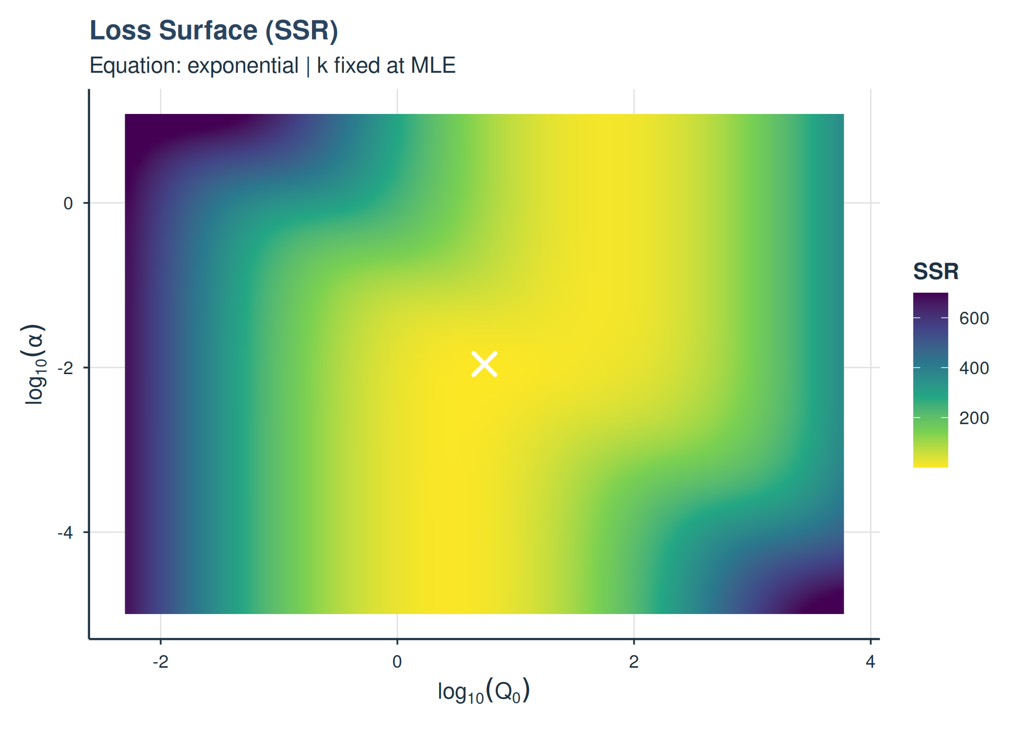

2D loss surface (SSR) over the Q0-alpha parameter space.

Profile plots show 1D slices through the loss surface, fixing one parameter at its MLE and varying the other:

plot_loss_profile(fit_2re)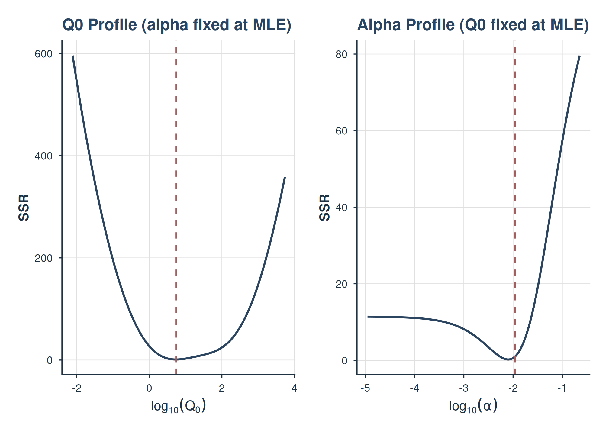

1D loss profiles for Q0 and alpha.

Subject Heterogeneity

Visualize the distribution of subject-level \alpha estimates to assess heterogeneity in price sensitivity:

plot_alpha_distribution(fit_2re)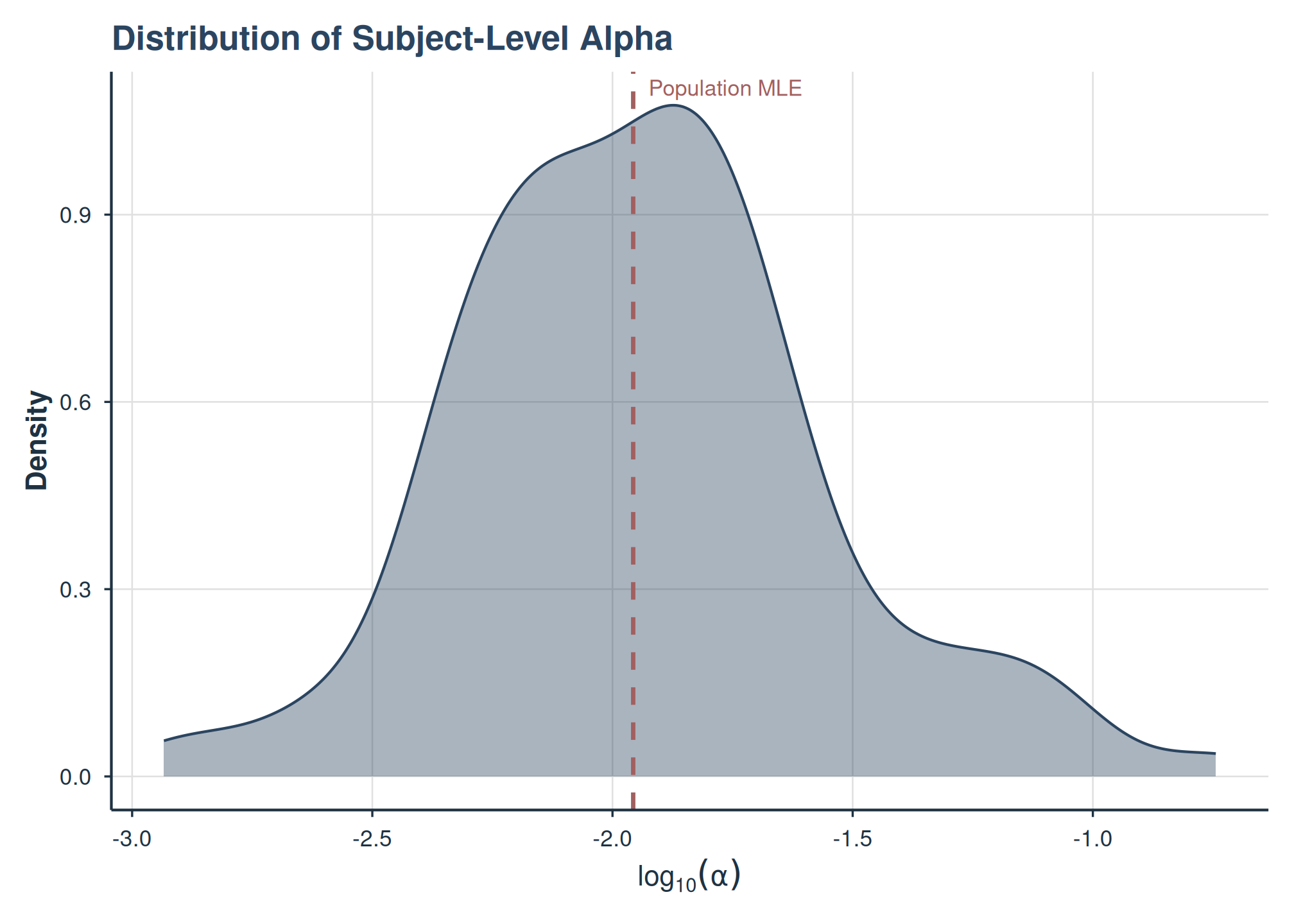

Distribution of subject-level alpha (elasticity) estimates.

Multi-Model Comparison

Overlay demand curves from multiple models to visualize how different specifications affect the predicted demand function:

plot_demand_overlay(fit_1re, fit_2re, labels = c("1-RE", "2-RE"))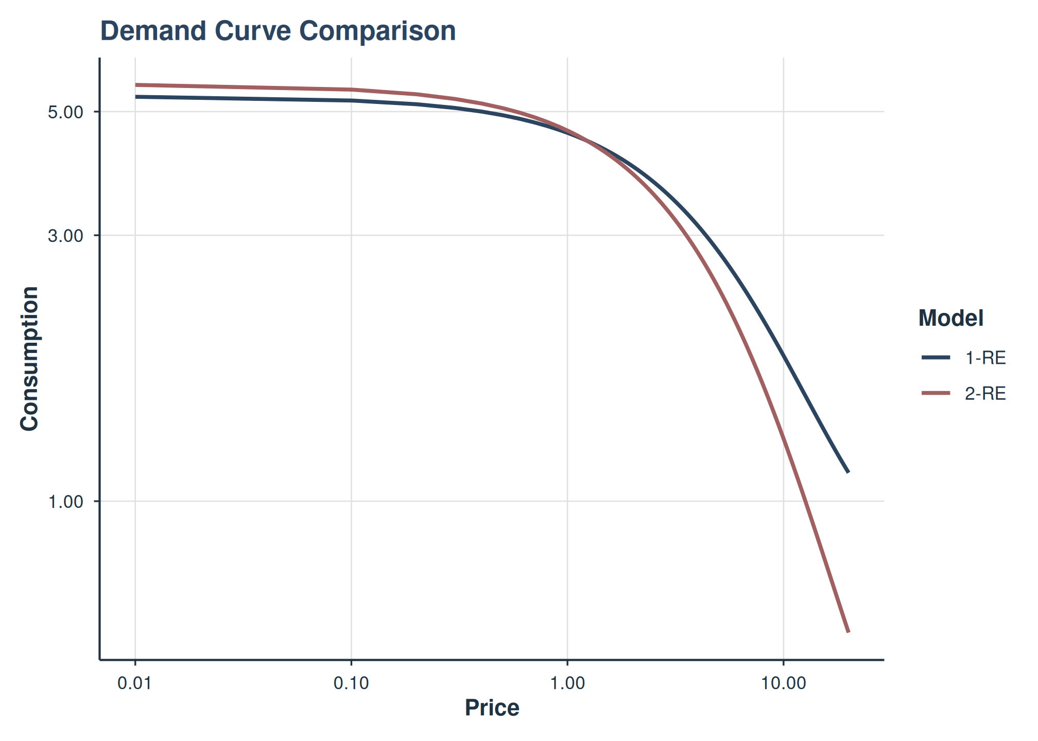

Demand curves from 1-RE and 2-RE models overlaid.

Compare parameter distributions side by side:

plot_model_comparison(fit_1re, fit_2re, labels = c("1-RE", "2-RE"))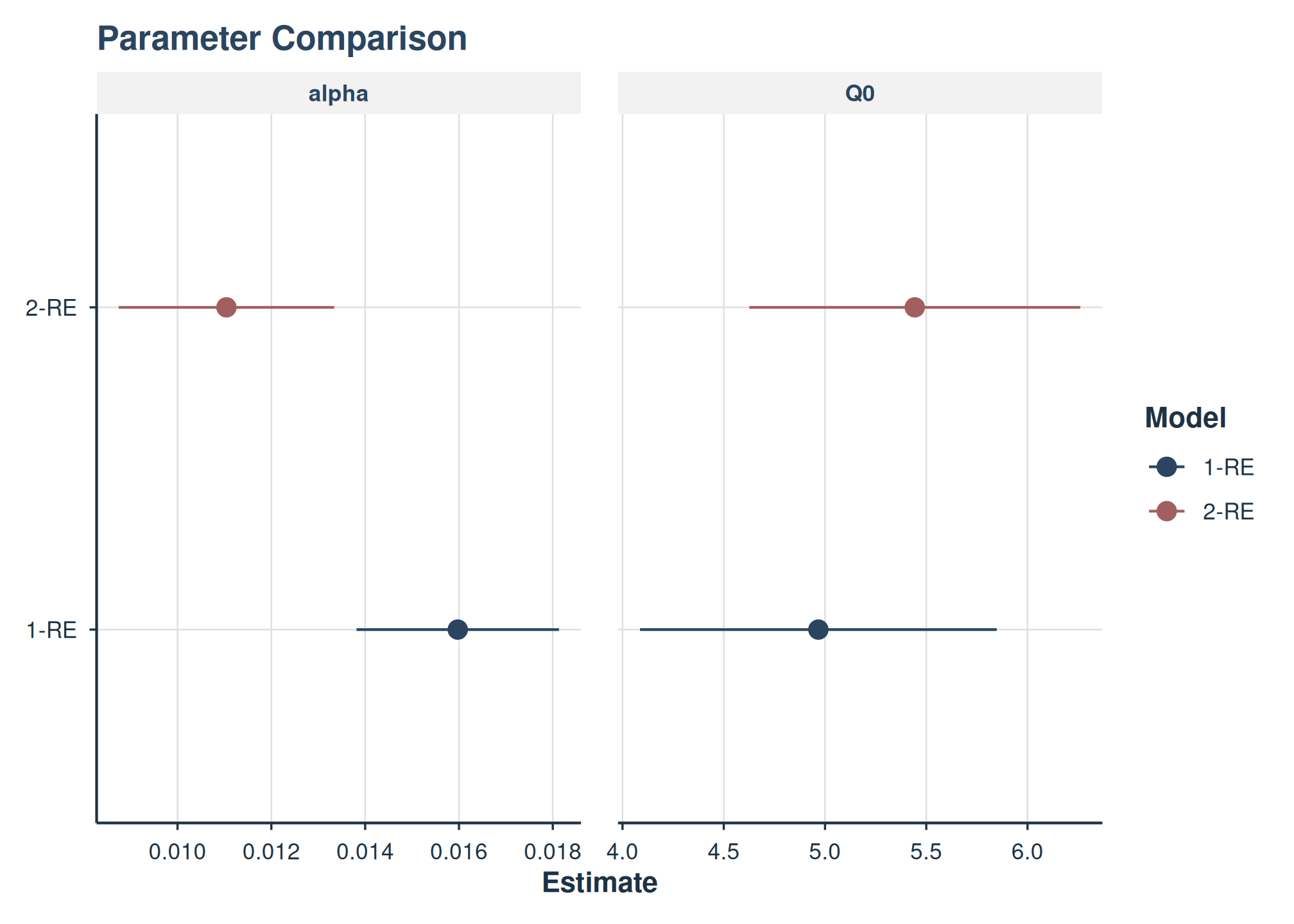

Side-by-side parameter estimates from 1-RE and 2-RE models.

Group Comparisons

To test whether demand parameters differ by group, pass factor variables via the factors argument. This adds fixed effects to the design matrices for both Q_0 and \alpha.

# Filter to Male/Female for a clean two-level comparison
dat_mf <- dat |> filter(gender %in% c("Male", "Female"))

fit_gender <- fit_demand_tmb(
  dat_mf,
  y_var = "y", x_var = "x", id_var = "id",
  equation = "exponential",
  factors = "gender",
  random_effects = c("q0", "alpha"),
  verbose = 0
)
fit_gender
#> 
#> TMB Mixed-Effects Demand Model
#> 
#> Call:
#> fit_demand_tmb(data = dat_mf, y_var = "y", x_var = "x", id_var = "id", 
#>     equation = "exponential", random_effects = c("q0", "alpha"), 
#>     factors = "gender", verbose = 0)
#> 
#> Equation: exponential 
#> Convergence: Yes 
#> Number of subjects: 99 
#> Number of observations: 1131 
#> Observations dropped (zeros): 569 
#> Random effects: 2 (q0, alpha) 
#> Log-likelihood: -267.38 
#> AIC: 552.76 
#> 
#> Fixed Effects:
#>       Q0.0       Q0.1    alpha.0    alpha.1      log_k   logsigma   logsigma 
#>     1.6093     0.1941    -4.4026    -0.2493     0.3404    -0.3021    -0.1074 
#> logsigma_e    rho_raw 
#>    -1.4905    -0.4591 
#> 
#> Use summary() for full results.

Joint Tests

anova(fit) reports a joint Wald-χ² test for each parameter × factor block — here, whether gender shifts Q_0 and \alpha. Pass additional fits for a nested likelihood-ratio test.

anova(fit_gender)
#> # A tibble: 2 × 4
#>   Group          Chisq    df p.value
#>   <chr>          <dbl> <int>   <dbl>
#> 1 Q0 ~ gender     1.61     1   0.205
#> 2 alpha ~ gender  1.63     1   0.202

Estimated Marginal Means

get_demand_param_emms(fit_gender, param = "Q0")
#> # A tibble: 2 × 6
#>   level         estimate estimate_log std.error conf.low conf.high
#>   <chr>            <dbl>        <dbl>     <dbl>    <dbl>     <dbl>
#> 1 gender=Female     5.00         1.61     0.102     4.10      6.10
#> 2 gender=Male       6.07         1.80     0.115     4.85      7.60

get_demand_param_emms(fit_gender, param = "alpha")
#> # A tibble: 2 × 6
#>   level         estimate estimate_log std.error conf.low conf.high
#>   <chr>            <dbl>        <dbl>     <dbl>    <dbl>     <dbl>
#> 1 gender=Female  0.0122         -4.40     0.133  0.00943    0.0159
#> 2 gender=Male    0.00954        -4.65     0.155  0.00705    0.0129

EMMs are reported on both the natural scale (estimate) and log scale (estimate_log). The natural-scale estimates represent the population-average Q_0 or \alpha for each group.

Pairwise Comparisons

get_demand_comparisons(fit_gender, param = "Q0")
#> Demand Parameter Comparisons (tmb backend)
#> EMMs computed over: all fitted factors 
#> Contrast type: pairwise
#> P-value adjustment method: holm 
#> ================================================== 
#> 
#> Q0 (log10-scale contrasts):
#>       contrast estimate std.error conf.low conf.high p.value
#>  Female - Male   -0.084     0.067   -0.215     0.046   0.205

get_demand_comparisons(fit_gender, param = "alpha")
#> Demand Parameter Comparisons (tmb backend)
#> EMMs computed over: all fitted factors 
#> Contrast type: pairwise
#> P-value adjustment method: holm 
#> ================================================== 
#> 
#> alpha (log10-scale contrasts):
#>       contrast estimate std.error conf.low conf.high p.value
#>  Female - Male    0.108     0.085   -0.058     0.275   0.202

The estimate_ratio column gives the multiplicative ratio between groups on the natural scale (e.g., a ratio of 1.34 means Group A’s Q_0 is 34% higher than Group B’s).

Factor interaction and continuous covariate sections are skipped in fast render mode. Set BEEZDEMAND_VIGNETTE_MODE=full to include them.

Model Comparison

Use compare_models() to compare nested TMB models via likelihood ratio test, AIC, and BIC:

compare_models(fit_1re, fit_2re)
#> 
#> Model Comparison
#> ================================================== 
#> 
#>    Model          Class   Backend nobs df    logLik       AIC       BIC
#>  Model_1 beezdemand_tmb TMB_mixed 1131  5 -639.5903 1289.1807 1314.3350
#>  Model_2 beezdemand_tmb TMB_mixed 1131  7 -268.5364  551.0729  586.2889
#>  delta_AIC delta_BIC
#>   738.1078  728.0461
#>     0.0000    0.0000
#> 
#> Best model by BIC: Model_2 
#> 
#> Likelihood Ratio Tests:
#> ---------------------------------------- 
#>          Comparison  LR_stat df p_value
#>  Model_1 vs Model_2 742.1078  2  <2e-16
#> 
#> Notes:
#>   - LRT nesting assumption not verified.

Valid comparisons require models fit on the same data with the same equation and response scale. Models with different equations (e.g., exponential vs exponentiated) model different responses and cannot be compared via AIC.

Building Nested Models with `update()`

update(fit, ...) re-fits with named arguments substituted into the original fit_demand_tmb() call. Use it to build a candidate fit and drop or add factors / covariates / random effects without typing the full fit call again:

# Drop the gender factor to test its joint significance:
fit_gender_null <- update(fit_gender, factors = NULL)
compare_models(fit_gender_null, fit_gender)
#> 
#> Model Comparison
#> ================================================== 
#> 
#>    Model          Class   Backend nobs df    logLik      AIC      BIC delta_AIC
#>  Model_1 beezdemand_tmb TMB_mixed 1131  7 -268.5364 551.0729 586.2889    0.0000
#>  Model_2 beezdemand_tmb TMB_mixed 1131  9 -267.3790 552.7580 598.0357    1.6851
#>  delta_BIC
#>     0.0000
#>    11.7468
#> 
#> Best model by BIC: Model_1 
#> 
#> Likelihood Ratio Tests:
#> ---------------------------------------- 
#>          Comparison LR_stat df p_value
#>  Model_1 vs Model_2  2.3149  2   0.314
#> 
#> Notes:
#>   - LRT nesting assumption not verified.

evaluate = FALSE returns the unevaluated call (for inspection) instead of re-fitting, matching the convention of stats::update.default.

formula(fit) and model.matrix(fit) round out the introspection API. formula(fit) returns a named list of one-sided formulas for Q0 and alpha plus the random-effect spec; model.matrix(fit) returns the four design matrices the TMB template consumed (X_q0, X_alpha, Z_q0, Z_alpha) — a named list rather than the single matrix lm or lme4 return, because the TMB tier truly has two fixed-effect linear predictors.

Convergence Tips

If a model fails to converge, try these strategies in order:

Strategy	How	When
Reduce random effects	`random_effects = "q0"`	2-RE models struggling
Use exponential equation	`equation = "exponential"`	Exponentiated/simplified not converging
Fix k	`estimate_k = FALSE, k = 2`	k estimate drifting to extreme values
Increase iterations	`tmb_control = list(iter_max = 2000)`	“false convergence” messages
Try L-BFGS-B	`tmb_control = list(optimizer = "L-BFGS-B")`	nlminb not making progress
Set parameter bounds	`tmb_control = list(lower = ..., upper = ...)`	Estimates at boundaries
Warm start	`tmb_control = list(warm_start = prev_fit$opt$par)`	Refining a near-converged fit

# Switch optimizer
fit <- fit_demand_tmb(
  dat, equation = "exponential",
  tmb_control = list(optimizer = "L-BFGS-B"),
  verbose = 0
)

# Warm-start from a previous fit
fit2 <- fit_demand_tmb(
  dat, equation = "exponential",
  tmb_control = list(warm_start = fit$opt$par),
  verbose = 0
)

# Apply parameter bounds
fit3 <- fit_demand_tmb(
  dat, equation = "exponential",
  tmb_control = list(
    lower = c(log_k = -2),
    upper = c(log_k = 4)
  ),
  verbose = 0
)

# Disable multi-start for faster iteration during exploration
fit4 <- fit_demand_tmb(
  dat, equation = "exponential",
  multi_start = FALSE,
  verbose = 2
)

tmb_control Options

Field	Default	Description
`optimizer`	`"nlminb"`	`"nlminb"` or `"L-BFGS-B"`
`iter_max`	1000	Maximum iterations
`eval_max`	2000	Maximum evaluations (nlminb only)
`rel_tol`	1e-10	Relative tolerance (nlminb only)
`lower` / `upper`	NULL	Named numeric bounds on log-scale parameters
`warm_start`	NULL	Starting values from a previous `fit$opt$par`
`trace`	0	Optimizer trace level

Choosing Between fit_demand_tmb() and fit_demand_mixed()

Feature	`fit_demand_tmb()`	`fit_demand_mixed()`
Backend	TMB (C++, automatic differentiation)	nlme (R, numerical gradients)
Equations	exponential, exponentiated, simplified, zben	zben, simplified
k parameter	Estimated or fixed	Not available
Random effects	1 or 2 (Q0, alpha)	Configurable via nlme
Convergence	Robust (AD + Laplace + multi-start)	Can struggle with nonlinear equations
Speed	Fast (compiled C++)	Variable
Post-hoc EMMs	`get_demand_param_emms()`	`get_demand_param_emms()` (via emmeans)
Factors/covariates	Design matrices	Formula-based

Prefer fit_demand_tmb() for new work. fit_demand_mixed() remains useful when you need specific nlme features like custom correlation structures or when working with existing pipelines.

References

Hursh, S. R., & Silberberg, A. (2008). Economic demand and essential value. Psychological Review, 115(1), 186–198.

Koffarnus, M. N., Franck, C. T., Stein, J. S., & Bickel, W. K. (2015). A modified exponential behavioral economic demand model to better describe consumption data. Experimental and Clinical Psychopharmacology, 23(6), 504–512.

Kristensen, K., Nielsen, A., Berg, C. W., Skaug, H., & Bell, B. M. (2016). TMB: Automatic differentiation and Laplace approximation. Journal of Statistical Software, 70(5), 1–21.

Brent Kaplan

2026-08-17

Introduction

Quick Start

Choosing an Equation

Mathematical Specifications

Random Effects Structure

Estimating vs. Fixing k

Examining Results

Summary and Coefficients

Subject-Specific Parameters

Amplitude–Persistence Decomposition

Confidence Intervals

Variance-Covariance and the Delta Method

Predictions

Population Metrics

Visualization

Diagnostics

Advanced Visualization

Expenditure and Elasticity

Loss Surface and Profile

Subject Heterogeneity

Multi-Model Comparison

Group Comparisons

Joint Tests

Estimated Marginal Means

Pairwise Comparisons

Model Comparison

Building Nested Models with `update()`

Convergence Tips

tmb_control Options

Choosing Between fit_demand_tmb() and fit_demand_mixed()

References

See Also

TMB Mixed-Effects Demand Models

Brent Kaplan

2026-08-17

Introduction

Quick Start

Choosing an Equation

Mathematical Specifications

Random Effects Structure

Estimating vs. Fixing k

Examining Results

Summary and Coefficients

Subject-Specific Parameters

Amplitude–Persistence Decomposition

Confidence Intervals

Variance-Covariance and the Delta Method

Predictions

Population Metrics

Visualization

Diagnostics

Advanced Visualization

Expenditure and Elasticity

Loss Surface and Profile

Subject Heterogeneity

Multi-Model Comparison

Group Comparisons

Joint Tests

Estimated Marginal Means

Pairwise Comparisons

Model Comparison

Building Nested Models with update()

Convergence Tips

tmb_control Options

Choosing Between fit_demand_tmb() and fit_demand_mixed()

References

See Also

Building Nested Models with `update()`