Overlay Demand Curves from Multiple Models

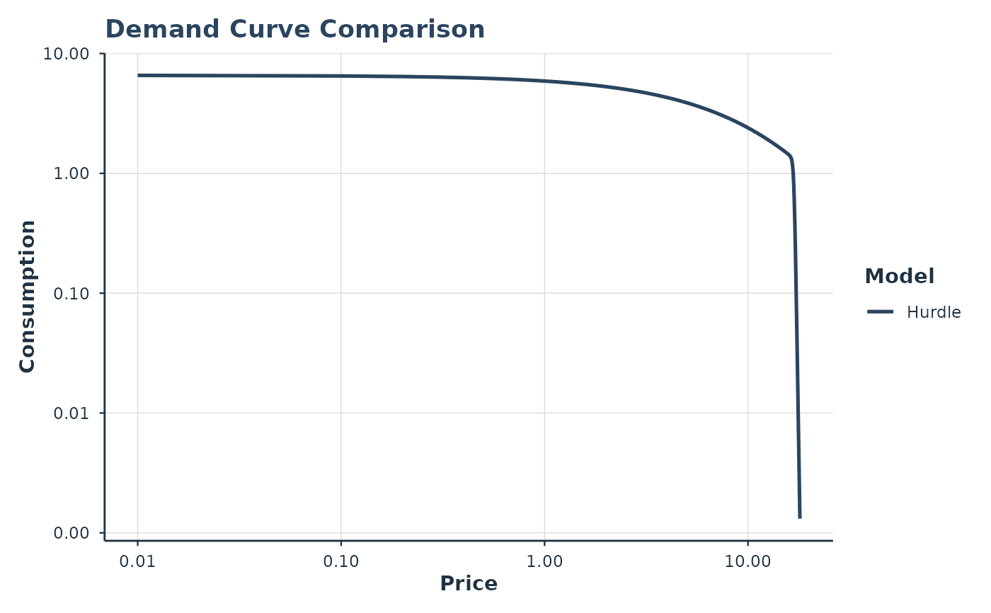
Plots population-level demand curves from multiple fitted models on the same axes for visual comparison.

Usage

plot_demand_overlay(
  ...,
  model_list = NULL,
  labels = NULL,
  prices = NULL,
  n_points = 200,
  x_trans = c("log10", "log", "linear", "pseudo_log"),
  free_trans = 0.01,
  y_min = 0.001,
  inv_fun = identity,
  x_lab = "Price",
  y_lab = "Consumption",
  style = c("modern", "apa")
)

Arguments

...

Fitted model objects (named or unnamed).

model_list

Optional named list of models (combined with ...).

labels

Character vector of model labels for the legend.

prices

Numeric vector of prices. Default uses the union of observed prices across all models.

n_points

Integer; number of points for smooth curves (default 200).

x_trans

Character; x-axis transformation (default "log10").

free_trans

Numeric; replacement for price = 0 on log scales.

y_min

Numeric; minimum consumption value to display. Values below this floor are dropped to prevent extreme predictions (e.g., 1e-16 from hurdle models) from compressing the y-axis. Set to NULL to disable. Default is 0.001.

inv_fun

Function to back-transform consumption values (e.g., ll4_inv for LL4-transformed models). Default is identity.

x_lab, y_lab

Axis labels.

style

Character; "modern" or "apa".

Value

A ggplot2 object.

Examples

# \donttest{
data(apt)
fit1 <- fit_demand_hurdle(apt, y_var = "y", x_var = "x", id_var = "id")
#> Sample size may be too small for reliable estimation.
#>   Subjects: 10, Parameters: 12, Recommended minimum: 60 subjects.
#>   Consider using more subjects or the simpler 2-RE model.
#> Fitting HurdleDemand3RE model...
#>   Part II: zhao_exponential
#>   Subjects: 10, Observations: 160
#>   Fixed parameters: 12, Random effects per subject: 3
#>   Optimizing...
#>   Converged in 81 iterations
#>   Computing standard errors...
#> Done. Log-likelihood: 32.81
# Compare with a 3-RE model:
# fit2 <- fit_demand_hurdle(apt, y_var = "y", x_var = "x", id_var = "id",
#   random_effects = c("zeros", "q0", "alpha"))
# plot_demand_overlay(fit1, fit2, labels = c("2-RE", "3-RE"))
plot_demand_overlay(fit1, labels = c("Hurdle"))

# }