Plot Expenditure Curves

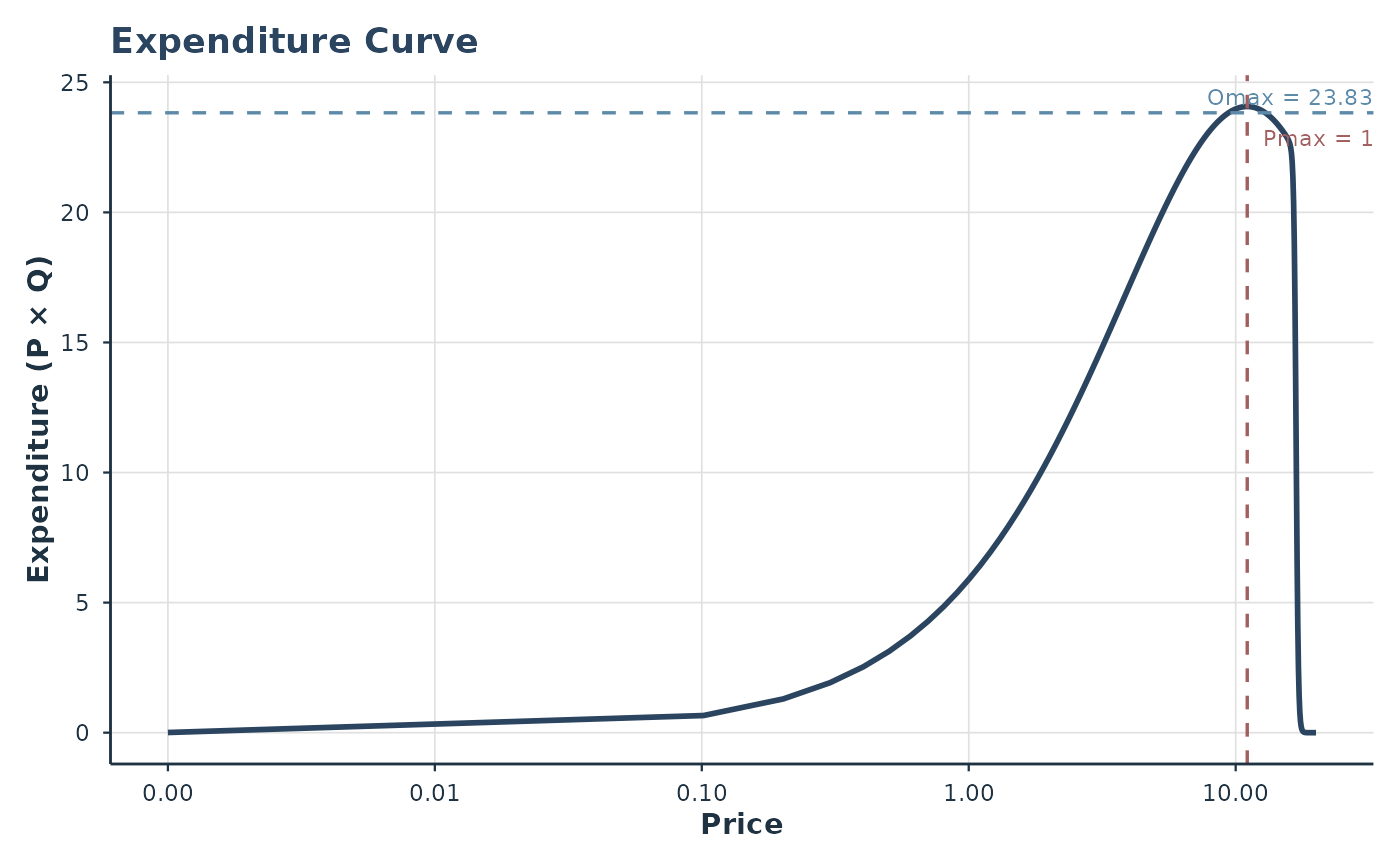
Plots the expenditure curve (Price x Consumption) derived from the fitted demand model. Optionally overlays Pmax and Omax reference lines.

Usage

plot_expenditure(object, ...)

# S3 method for class 'beezdemand_hurdle'
plot_expenditure(
  object,
  prices = NULL,
  n_points = 200,
  show_pmax = TRUE,
  show_omax = TRUE,
  demand_type = c("unconditional", "conditional"),
  x_trans = c("log10", "log", "linear", "pseudo_log"),
  free_trans = 0.01,
  x_lab = "Price",
  y_lab = "Expenditure (P × Q)",
  style = c("modern", "apa"),
  ...
)

# S3 method for class 'beezdemand_tmb'
plot_expenditure(
  object,
  prices = NULL,
  n_points = 200,
  show_pmax = TRUE,
  show_omax = TRUE,
  x_trans = c("log10", "log", "linear", "pseudo_log"),
  free_trans = 0.01,
  x_lab = "Price",
  y_lab = "Expenditure (P × Q)",
  style = c("modern", "apa"),
  ...
)

Arguments

object

A fitted model object.

...

Additional arguments passed to methods.

prices

Numeric vector of prices. If NULL, uses a smooth grid spanning the observed price range.

n_points

Integer; number of grid points (default 200).

show_pmax

Logical; show Pmax vertical line (default TRUE).

show_omax

Logical; show Omax horizontal line (default TRUE).

demand_type

Character; for beezdemand_hurdle only. "unconditional" (default) plots p * (1 - P0(p)) * Q(p) and overlays the unconditional Pmax/Omax reference lines. "conditional" plots the Part-II demand p * Q(p) (consumption given positive purchase) and overlays the Part-II-only Pmax/Omax reference lines. Either way the displayed curve and the Pmax/Omax lines are guaranteed to come from the same metric set, so they always align.

x_trans

Character; x-axis transformation (default "log10").

free_trans

Numeric; replacement for price = 0 on log scales.

x_lab, y_lab

Axis labels.

style

Character; "modern" or "apa".

Value

A ggplot2 object.

Examples

# \donttest{
data(apt)
fit <- fit_demand_hurdle(apt, y_var = "y", x_var = "x", id_var = "id")
#> Sample size may be too small for reliable estimation.
#>   Subjects: 10, Parameters: 12, Recommended minimum: 60 subjects.
#>   Consider using more subjects or the simpler 2-RE model.
#> Fitting HurdleDemand3RE model...
#>   Part II: zhao_exponential
#>   Subjects: 10, Observations: 160
#>   Fixed parameters: 12, Random effects per subject: 3
#>   Optimizing...
#>   Converged in 81 iterations
#>   Computing standard errors...
#> Done. Log-likelihood: 32.81
plot_expenditure(fit)

# }